Additional Modes

This chapter describes other Artec Studio modes, such as

Publishing to the Web

Having models on a web may simplify the process of collaboration among users. Artec Studio allows you to publish your 3D models on the Web through viewshape.com. Viewshape is a service that uses WebGL to render 3D models in a web browser. You can see published models at viewshape.com or embedded at other websites, blogs or social networks. Models can be shared privately so that only those who know the unique URL can see, comment on and use them.

Most browsers currently support WebGL. If this feature is disabled or unsupported in a particular browser, viewshape.com displays the 3D geometry as a pre-rendered set of images that you can rotate using a mouse. Such images are called spin images.

To publish a model, use the Publish panel. It will open only if you have exactly one fusion selected in the Workspace window; otherwise, Artec Studio will display an error message. To log into viewshape.com, use your my.artec3d account. If the process fails, you can access the login window from the link at the top of the panel (see Figure 116).

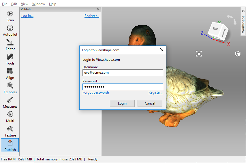
Figure 116 Viewshape.com login window.

After you successfully login, you will see the window shown in Figure 117. Follow the steps below to continue uploading:

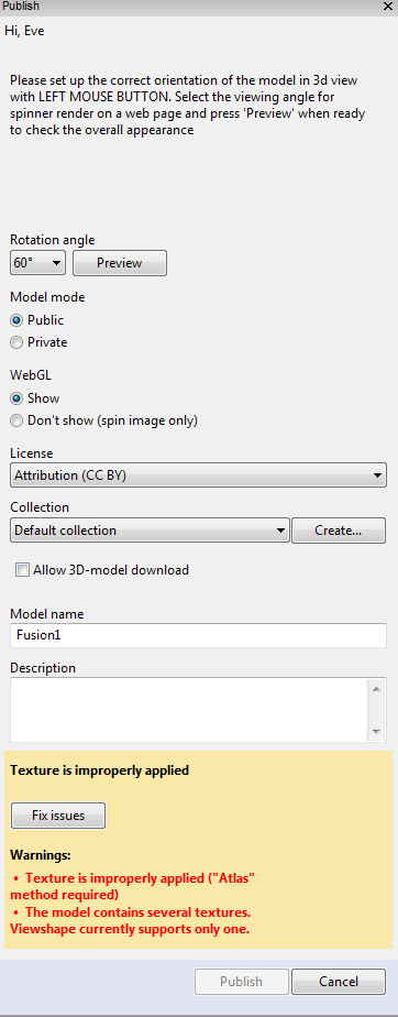
Figure 117 Publish panel.

1. Adjust model’s position in the 3D View window to see how it will appear on the Web.
2. Preview rotation when necessary.
3. Select visibility options (Public or Private).
4. Choose whether to employ WebGL: use Show to display a full-featured 3D model and rotate it freely, or use Don’t show (spin image only) to display images of the model captured from different angles. You can rotate these images only around the vertical axis.
5. Select a license type for your model.
6. Specify the collection in your gallery to which you want to publish the model, or create a new one.

In addition to the above steps, you must also set the Model name and, optionally, the Model description. Once you have completed this entire process, click Publish; your model will appear on the site.

Model Requirements

WebGL is a progressive API, but it is not very powerful. If your model contains several million polygons and several very high-resolution textures, you will have difficulty rendering it in a browser. Therefore, to produce a model that looks good, you must first optimize it. We recommend the following model parameters:

• Fewer than 1000000 polygons
• Texture size of 4096×4096 pixels
• Texture mapped using Atlas method (mandatory)
• Model positioned appropriately to rotate around Y axis

Using LMB in the 3D View, you can rotate the model around its center of mass. Because translation is impossible here, you should rotate the model to the position in which you want it to appear on the web.

If the model parameters fail to satisfy the requirements and recommendations listed above, a yellow notification will appear at the bottom of the window, along with a button that instructs Artec Studio to fix the issue.

Fixing Issues

If your model suffers from one or more issues (as Figure 117 shows), click the Fix issues button. The software will open the new panel shown in Figure 118.

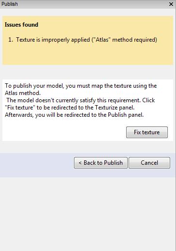
Figure 118 Fixing model issues.

Artec Studio can currently identify two issues: very dense meshes and incorrect texture mapping. If the mesh is too dense, you must first simplify the model. The simplification tool is available in the Issues found dialog. If the texture is mapped using the Preview method (triangle map), you can remap it by clicking Fix texture, as Figure 118 shows. The Texture panel will then open, allowing you to fix it using the Export method (texture atlas) and the recommended resolution.

Once you have resolved all the issues, click Back to Publish to return to the Publish panel and resume the publication process.

Multicapturing

Artec Studio enables synchronized scanning with multiple scanners. This mode is helpful when capturing a large object from several angles using more than one scanner simultaneously. Multicapturing with several scanners implies that the system knows their position in advance. This condition simplifies and accelerates data processing considerably. For this reason you must calibrate the relative positions of the scanners before capturing. The resulting calibration data, which includes scanner IDs and their spatial orientations, is referred to as a bundle.

You can bundle Artec 3D scanners, third-party 3D sensors or any combination thereof. The only restriction is that the bundle should include no more than one Microsoft Kinect v2 or Intel RealSense (F200, R200 or SR300) device.

Important

Using multiple Artec scanners requires your workstation to integrate as many independent USB host controllers as connected scanning devices.

Note

Also note that adding a third-party 3D sensor to a bundle is only possible in Artec Studio Ultimate.

Use the following procedure to prepare the devices and the environment to simultaneously capture 3D reality:

1. Calibrate the relative position of each device (i.e., create a bundle)
2. Use the Multi panel to capture scans

To create a bundle, perform the following steps:

1. Capture the test object using all bundled scanners (see object requirements in Bundle Creation)
2. Manually align the resulting scans using the Align tool to compute the relative position of all scanners
3. Create the bundle using the Create bundle panel

Note

Once you have created the bundle, you can no longer move the scanners relative to one another. If even one device has changed position, you must recreate the bundle!

Bundle Creation

Perform the following steps before creating a scanner bundle:

1. Select device positions. The scanners’ combined field of view should cover the required area.
2. Fix the scanners in the chosen positions. If you plan to use hardware synchronization (see EVA Scanners: Hardware Synchronization), attach the scanners to the tripods by securing them with thumbscrews while allowing the wires to hang freely.
3. Select and set up the calibration object. Any object with a geometry-rich surface is a candidate. Avoid selecting objects with simple geometries for calibration (e.g., planes, spheres or cylinders). You may use several objects as a composition when creating a bundle. We recommend object installation at the distance corresponding to the middle of the operating range for the corresponding device type.

You can perform the scan using the Capture or Multi panel. The latter option is more convenient, as it allows you to capture the video data stream simultaneously from several scanners. For details regarding this mode, see Performing Multicapture.

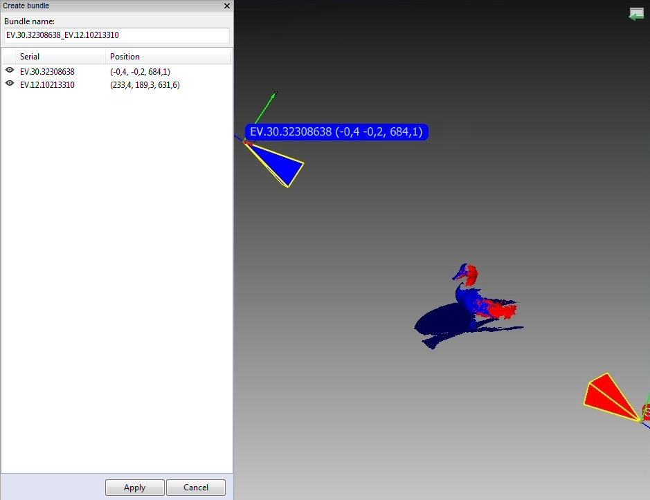
Figure 119 Bundle-creation window.

If you install the scanners at small angles relative to each other (i.e., you can see the same object area simultaneously through different scanners), you need not rotate the object. In this case, you can take calibration scans either sequentially or concurrently.

Note

In case of sequential scanning, make sure the object is fixed safely and remains motionless during the scan.

If you set up the scanners at a large angle and their fields of view have no overlap, use the Multi panel to start the capture sequence and then turn (move) the object to enable all scanners to capture the same parts.

Note

It is important that all scanners capture a large portion of the object or scene (but not necessarily the same portion) in each frame, because the position of all subsequent frames—as well as the scanners themselves—will be determined by their predecessors. Also, the relative positions of the scans will determine the intercalibration of the devices.

If the cameras are far from each other and the object was moving, then you should register the scans using the Fine registration and Global registration algorithms. This requirement, however, isn’t applicable for 3D sensors: running Global registration may spoil the scans owing to low quality of the geometry obtained from the sensors.

4. Next, proceed to the Align panel and align the captured scans as Scan Alignment describes. At that point, everything will be ready for bundle creation.
5. From the menu, select File → Create bundle. A warning message will appear if you forget to align the scans. Otherwise, the bundle-creation panel will appear (see Figure 119). The 3D View window will show the selected scans, the position and viewing direction of the scanners (by means of an appropriately colored pyramid), the device ID, and the scanner coordinates. It will display a list of connected devices and corresponding information.
6. Add a device to the bundle or remove one by inverting the image in the leftmost column of the list. The order of devices in a bundle refers to the scan order in the Workspace panel.
7. A bundle name will appear in the field at the top of the bundle-creation panel. By default it contains the serial number of the bundled scanner. Before creating the bundle, you can easily change this name by typing in the corresponding field. Click Apply at the bottom of the panel to create and install the bundle.

Performing Multicapture

Multi mode allows you to capture 3D-data streams simultaneously from several devices. Selecting this mode activates the corresponding panel (see Figure 120) and lets you choose the device configuration: either use one of the existing bundles or specify the scanner list manually.

Note

In multicapture mode the system possesses information about the relative scanner positions. Therefore, scans captured by bundled scanners differ from manual scans in that the matching frames from different scanners are already in the same coordinate system.

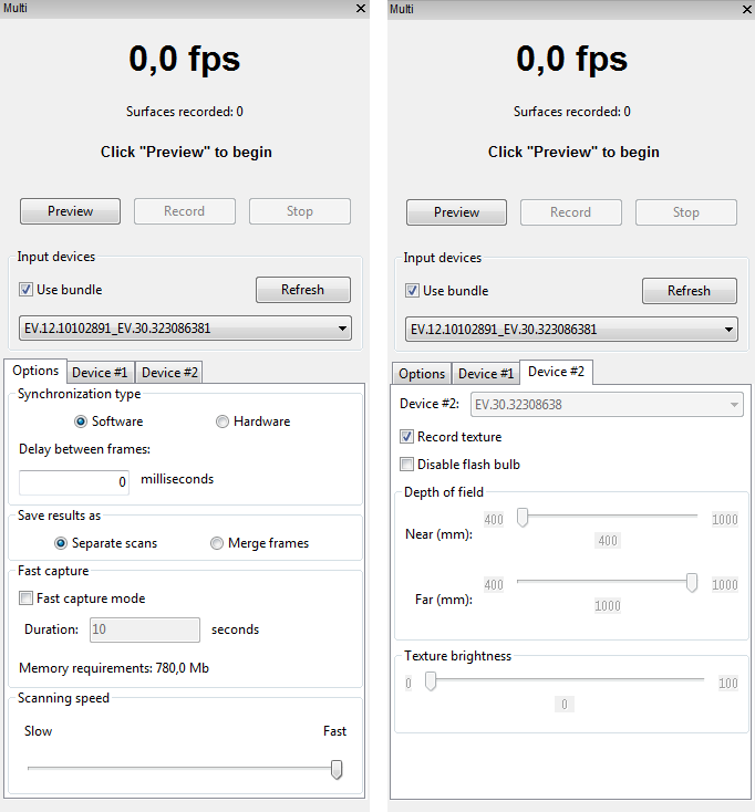
Figure 120 Multicapture panel: Options tab on left, Device tab on right.

1. Select the Use bundle checkbox. A dropdown list of all installed bundles will appear in the panel. Active bundles are highlighted in black, inactive bundles in gray. Artec Studio considers the bundle active if all bundled devices are installed and connected to the PC.

2. Select Synchronization type from the Options tab in the Multicapture panel.

   • In Software mode, scanners are synchronized via USB, Windows and Artec Studio, and the slave-scanner actuation time always varies (~10 milliseconds) owing to the numerous links in the chain.
   • In Hardware mode, scanners are synchronized via cables (see EVA Scanners: Hardware Synchronization for details). Hardware synchronization provides high precision and repeatability for slave-scanner actuation time (about 1 millisecond with a precision of less than 10 microseconds, thanks to microelectronic processes).

   Note

   We recommend hardware synchronization in most circumstances; when capturing moving objects, it is mandatory.

3. Click Preview to start capture.

Tweaking Multicapture Options

You can store multicapture data either as separate scans (use the Separate scans radio button) or as a single scan in which every frame represents an aligned union of corresponding frames from all bundled devices (use the Merge frames radio button).

If you need to capture frames with a certain delay between the scanners, enter the delay value in the Delay between frames field. Unlike the Scan mode, the Multicapture mode captures each frame independently without attempting to align each subsequent frame with the previous one, so it makes sense.

Sometimes, limiting the cameras’ field of view is necessary (e.g., to cut off extraneous distant objects). Two sliders in the Depth of field area set the near and far scanning boundaries. The application sets work-area boundaries for each device independently in the device tabs (see Figure 120, right). By default, the minimum and maximum boundary values for the corresponding device type are set to the recommended range; we encourage you to avoid changing them. However, if you’re using Artec L scanners or 3D sensors, it may become necessary. To change these values manually, mark the Override default depth range checkbox in the Scan tab of the Settings dialog and enter the appropriate values in the fields below.

Note

For most scanner types, redefining the recommended depth range may reduce accuracy.

Fast capture mode instructs Artec Studio to store raw scanned data in memory and processes frames after completing the capture sequence. It allows to save processor time on building and rendering surfaces. And if the number of processor cores is less then doubled number of scanners in the bundle, it can also increase scanning speed.

To enable it,

1. Check the Fast capture mode box.
2. Enter the desired capture duration in seconds. The application will automatically recalculate and display the required amount of memory.

Artec Studio saves multicapture parameters when you exit the application and reapplies them the next time you start it.

Measurement Tools

Artec Studio offers a number of measurement and commenting tools, including

• Linear measure
• Geodesic measure
• Sections (cross-sections)
• Surface-distance maps
• Annotations

The corresponding buttons reside in the upper part of the Measures panel (see Figure 121).

1. Choose a measurement tool, the application displays a list of scans you can work with
2. Select the checkbox of each desired scan. The scans will appear in the 3D View window.
3. Click Next. The selected measurement-tool window will open.

The coverage below takes a closer look at the different measurement tools and their features.

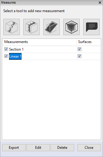
Figure 121 Measures panel.

Hint

If your Measurement panel lists the previously created items, you can open one of them by double-clicking that item or clicking the Edit button.

Linear Distance

The linear-measurement tool (see Figure 122) allows you to measure distances between selected points and to measure the total length for a string of multiple points. Click the button and select the scan to switch to the Linear window. You can enter a name for the new measurement by typing it in the Name field in the upper part of the window. The application creates new measurements with default names Linear 1, Linear 2 and so on.

To measure distances between points,

• Use LMB to sequentially select the points on the model in the 3D View window. The application will add these points to the current point list, which will also display linear dimensions and point coordinates.

• When you roll the cursor over any one of these points in the 3D View window, the point will be highlighted in red; you can then drag it to another location using LMB. When you release the mouse button, the point will fix to its new location.

  Warning

  You can’t set a point outside the object’s surface; in this situation, if you release the mouse button, the point will return to its original position.

The total number of points and total length of the measurements appear in the Measures panel.

Table 15 Basic operations in the linear and geodesic measurement modes.

Purpose	Control Name
Hide scans in the 3D View	Hide source data checkbox
Display order numbers of points	Show numbers checkbox
Display dimension results in the 3D View	Show labels checkbox
Specify the label and line color	Color button
Start a new measurement chain on the same objects (clear 3D View of all points and empty point list)	Make another button
Export measurements in a CSV or XML file	Export button
Return to the original Measures tab	Measurements link in the upper part of the panel

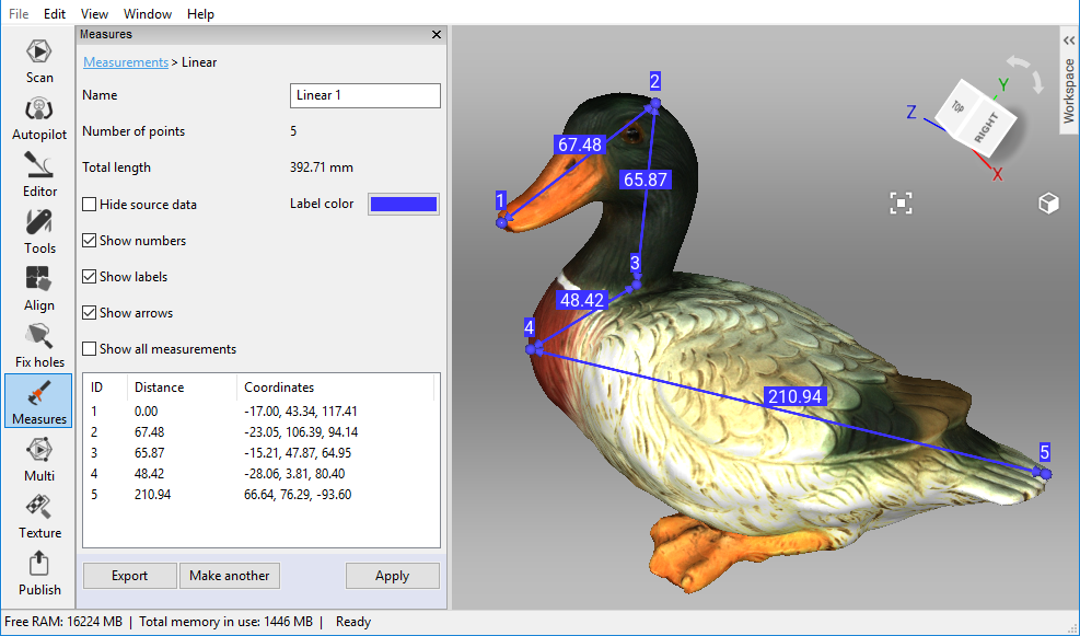
Figure 122 Linear measurement.

After you click Apply, the application will return to the original Measures panel and will display a list of all saved measurements along with editing and deletion options.

Geodesic Distance

Geodesic distance is defined as the length of the shortest path over a surface between several given points. Click the button in the Measures panel and select a point-cloud scan or model to start using the tool.

Working with geodesic measurements is similar to working with linear measurements (see Figure 123). Calculation of the shortest path is a time-consuming process that is accompanied by a progress-bar window. Also keep in mind that the shortest path between different surfaces or disconnected parts of the same surface is not defined. Therefore, the program will display an error if you select points on parts of a surface that are not connected to each other.

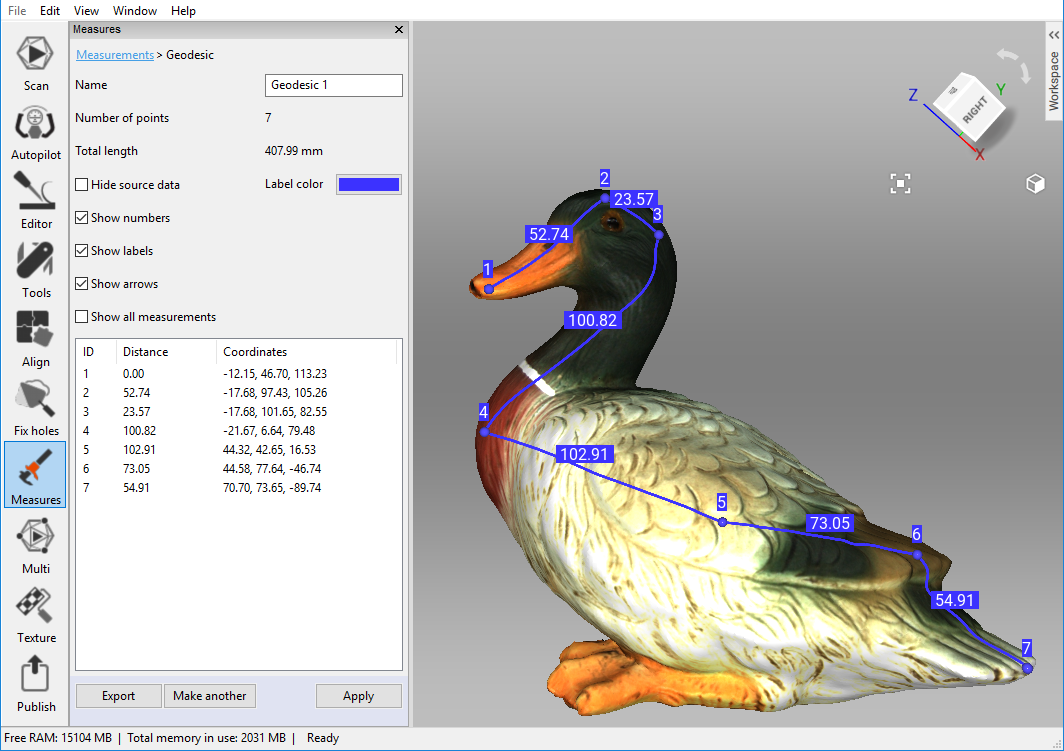
Figure 123 Geodesic-distance measurement.

Note

The geodesic algorithm is complex, and computations for a large number of vertices may take a long time. Therefore, if you choose the first point on a surface containing more than 150000 points total, the software will warn you that it may be a lengthy operation. You can either use the mesh-optimization algorithm beforehand (see Mesh Simplification) or delete the parts of the surface that you don’t need.

The left panel in this mode is similar to the one for linear-measurement mode (see Linear Distance).

Using Sections to Measure Area and Volume

Section is the plane that splits model or scan into two parts. Once created, it can provide you with data on volumes and areas of these parts as well as area and perimeter of the contour, i.e. the line formed as an intersection of the plane with surface.

To create a section of the object, follow the steps:

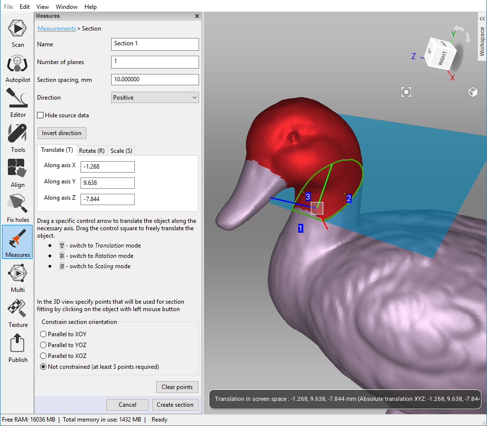
Figure 124 Orienting new section in Translate mode.

1. Click the button in the Measurements panel and select one or more models or scans. Models are preferable, since they contain only one surface.

2. Click Next and change the section name in the Name field as necessary.

3. Select constrain type in the bottom of the panel: Parallel to either plane or Not constrained

4. Use LMB to mark points on the object’s surface:

   1. Mark only one point to specify a plane in parallel with one of the coordinate planes (XOY, YOZ, XOZ).
   2. Mark three points to specify the plane that passes through them exactly.
   3. Mark more than three points to specify the plane that passing through their center of mass.

5. Redefine your point selections, if necessary, before you use Create section; to do so, click the Clear points button.

6. Orient plane position as necessary. Choose a tool: Translate, Rotate or Scale. You can either specify numerical values (in the global coordinate system) in the text fields or drag the controls (see Figure 109, Figure 110 and Figure 111) in the 3D View window. For instance, enlarge Scale to make the plane cross the whole surface.

7. Click Create section.

8. Create a series of sections, if desired. To do so,

   1. Click the Change position button.
   2. Specify the quantity of planes you want to create by entering the value in Number of planes and define the spacing in the Section spacing, mm field.
   3. Then select from the Direction list one of three directions (Positive, Negative or Both) in which to create the new planes [1].

9. Save your changes by clicking Apply, or click Measurements in the upper part of the panel. To save the changes and begin creating the next plane, click Make another section.

[1]	If you want to separate a set of sections into individual ones, click Convert to multiple sections. The software will notify you that the operation was successful, and the new objects will appear in the Measurements list.

Once you have created the section, the Section panel will display its geometrical information. This information includes perimeter and area for contours as well as area and volume for parts of meshes. Besides displaying geometrical values, Artec Studio will show a list of meshes and contours that allows you to highlight them in the 3D View window.

Switching Selections

A section splits model into two parts (selections). Artec Studio displays volume and area of the one highlighted in red. To display volume or area of another part, click Invert direction.

To determine volume or area of the entire model, put down both values and sum up them. You can also move your plane in order to situate it below the model (see the step about orienting plane in the procedure above). This operation will highlight the entire model in red and display the corresponding calculations.

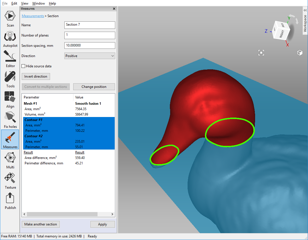
Figure 125 Using sections.

Comparing Values

The Section panel allows you to compare contours and mesh parts. To this end, select either two contours or two mesh parts from the list using the Ctrl key. Artec Studio will calculate the differences between the areas and perimeters of the contours and the difference between volumes and areas for mesh parts. These values will be available in the lower part of the Section panel (see Figure 125).

Exporting Sections

You can export sections in the following formats: CSV, XML or DXF.

• To export each section individually, enter the Section panel and click Export
• To export several objects at a time, access the original Measures panel, select the checkbox next to desired sections and then click Export.

Displaying Only Sections

To display only planes and contours, select the Hide source data checkbox.

Surface-Distance Maps

You may often find it necessary to compare two models and assess the deviation of their forms. For instance, quality control may require comparison of the original model with the scanned one. You can handle these tasks by using Surface-distance map.

Note

Artec Studio can only compare models or scans containing a single surface.

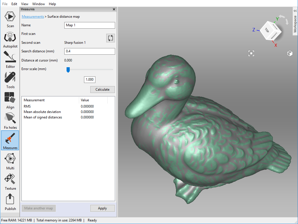
Figure 126 Specifying parameters for surface-distance map calculation.

Use this tool as follows:

1. Click the button from the Measures panel.

2. Select two models for comparison and click Next.

3. If necessary, specify the name of the distance map in the Name field of the Measures panel (see Figure 126). By default the application creates new distance maps under the names Map 1, Map 2 and so on.

   Note

   The direction along the normals of the first scan is considered positive; the opposite direction is considered negative. The button swaps scans.

4. Specify the Search distance (mm) value, a maximum range in millimeters for calculating distances between surfaces. You can adjust the actual range subject to this maximum after the calculation finishes.

5. Click Calculate. Once the process is complete, the distance map will appear in the 3D View window and the calculation results in the Measures panel (see Figure 127).

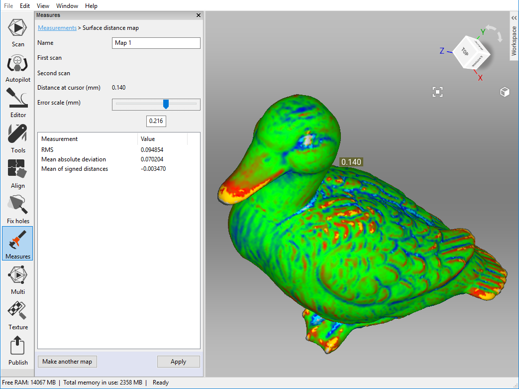
Figure 127 Surface-distance map calculated for two models.

You can analyze the calculation results and the distance map:

• On the basis of the Search distance value you entered, Artec Studio calculates the following:

  • RMS (root mean square)—the square root of the arithmetic mean of the squared distances
  • Mean absolute deviation
  • Mean of signed distances

• A distance map is a colored rendering on the particular surface regions. You can read the corresponding distance values and their distribution from the graduated scale and histogram that appear adjacent to the model. The map color changes from blue, which corresponds to a negative distance, to red, which corresponds to a positive distance.

  • Green means the distance between surfaces in this region is close to zero.
  • Gray highlights any surfaces with distances that exceed the specified Search distance.
  • Orange and bright blue correspond respectively to distances that are slightly above and below the limiting values of the scale.

• The graduated scale ranges from the positive value to the negative value of the Error scale. You can adjust this range using the Error scale (mm) slider or text box. Its maximum value cannot exceed the Search distance.

• If you move the mouse cursor to a particular point on the map, the exact distance will appear nearby and in the Distance at cursor field in the left panel.

To save the current distance map and quit this mode, click Apply. To save the current map and create another one, click Make another map.

Note

Surface-distance maps are supported by annotations. You can use any saved distance map in Annotation mode (see Annotations).

Annotations

Annotations tools allow you to mark noteworthy surfaces and surface-distance maps. The annotation can include one or more labels, which look like rectangular tags with connecting lines pointing to the corresponding surface elements (see Figure 128).

To create an annotation,

1. Click the button in the Measures panel, then select one or more scans and click Next.

   1. If you want to annotate a previously obtained surface-distance map, select it from the Distance map list.

2. Specify the Annotation name in the upper part of the panel, or simply proceed with your annotation using the default name.

3. Click LMB on the surface’s target point in the 3D View window; the label will appear with a blinking text cursor in the Annotation text field of the Measures panel.

   Note

   Artec Studio doesn’t enable you to redefine a label’s target point. If you inaccurately specify a point on the surface, add a new one (repeat Step 3) and delete the old one (consult the instructions below).

4. Type any desired text for your annotation; this text will appear in both the corresponding field in the panel and the label in the 3D View window.

5. Repeat Steps 3 and 4 to create a new label. In addition to tagging the surface, each new label will appear in the annotation list of the Measures panel (see Figure 128). You can show or hide labels in the list or change their colors by clicking RMB and selecting the appropriate option from the menu. Alternatively, toggle the selection flag or click the square button to show/hide labels or change their colors, respectively.

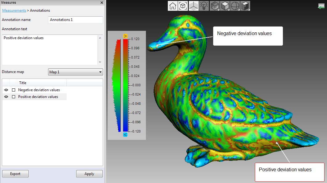
Figure 128 Annotation of a model layered with a surface-distance map.

You can adjust the label position (meaning the rectangular tag, not the target point!) by holding LMB in the 3D View window while moving the mouse cursor. To delete unnecessary labels, use any of the following approaches:

• Select the label in the 3D View window; its border color will become red (see selected label in Figure 128). Hit the Del key.
• Select the label from the list, then either hit Del, or click RMB and choose Delete from the menu.

To export annotations (more precisely, label coordinates and titles) to a CSV or XML file, click Export in either the Annotations or original Measures panel. By default, the file name will be the same as the annotation name. Accept it or type in another name of your choice. To complete the annotation, click Apply in the bottom of the Measures panel or click Measurements in the upper part.