Viewing Scans and Models

3D Navigation

When you have finished scanning, Artec Studio displays the results in the 3D View window.

Moving, Rotating and Scaling

You can control the observer’s perspective in the 3D View window by moving or rotating the observation point, or by zooming in or out. Use the mouse to control these effects.

Tip

You can also use 3D mouse to navigate 3D content (see 3D Mouse).

Moving

Move the mouse pointer over the 3D View window. Hold down the left (LMB) and right (RMB) mouse buttons simultaneously, then move the mouse to relocate the model. You can also use the middle mouse button to perform the same operation.

Rotating

To rotate around any possible axis, move the mouse pointer over the 3D View window. While holding down LMB, move the mouse in the desired direction to rotate the model.

Flipping

To quickly rotate (flip) 3D data around a specific axis (or rather the axis perpendicular to the screen plane) in a specific direction, use the dedicated arc arrows () near the navigation cube (see Figure 70) or the O key:

Using arrows

1. Click (LMB) one of the arrows ().
2. Still holding down LMB, move the mouse cursor in the direction of either of the arrows.

Using the O key

Press and hold the O key and drag the mouse cursor outside an imaginary ellipse that inscribes the 3D View window.

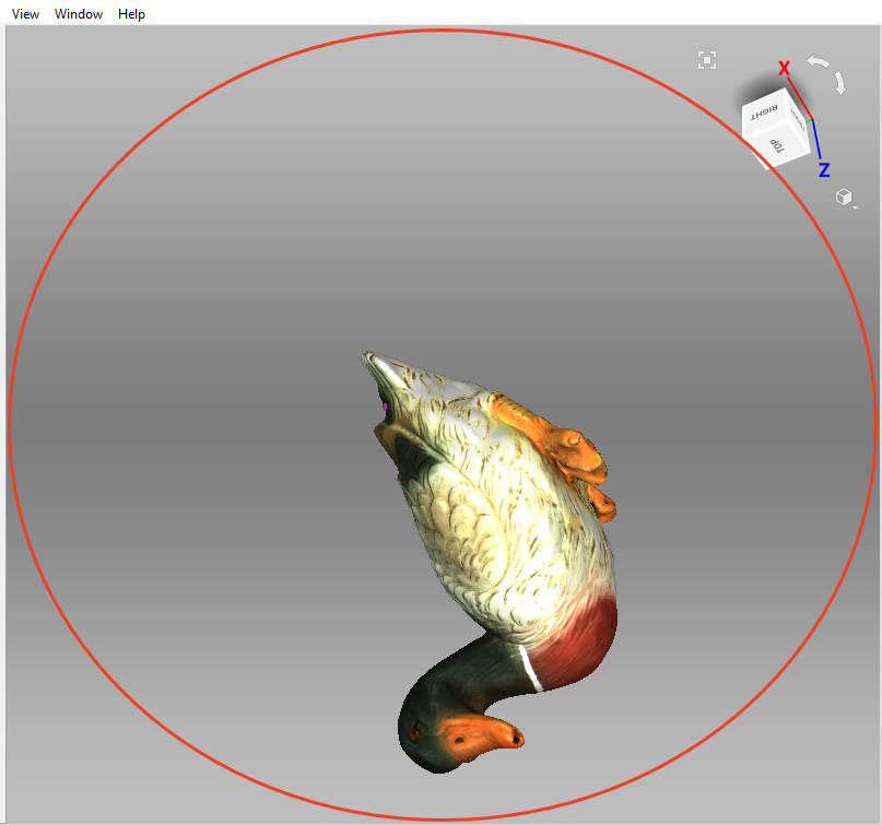
Figure 67 Imaginary ellipse inscribing the 3D View window.

Zooming

Hold RMB and move the mouse. Moving left or up will zoom out, whereas moving right or down will zoom in. You can also use the mouse wheel to produce the same effect.

Global Coordinate System and Rotation Center

To enable or disable the global coordinate-system axes, select the Show grid option in the View menu or Grid in the 3D View toolbar, or press G.

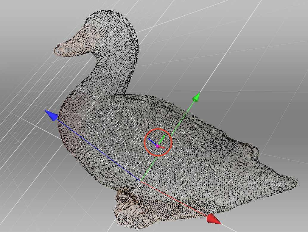
Figure 68 Custom rotation center.

When you rotate the model, the scene always turns around a certain point—the rotation center. By default, the rotation center coincides with the origin of the main axis grid. To change its location, double-click LMB at any point on the 3D model: the rotation center will move to this point. Setting the rotation center can be useful when you wish to view a particular object from all sides. Once it is set, rotate the view using LMB.

Artec Studio displays the rotation center as a small purple sphere with the three small coordinate axes (see Figure 68). If the rotation center coincides with the origin of the main axis grid, the purple sphere lacks small axes. If the rotation center hasn’t been altered, it even lacks the sphere.

Application can set the rotation center to the center of mass of the object. Access the following menu command: Edit → Cursor → Set to mass center. To go back to the default state, select Set to origin of axis grid.

Choosing Projections

The View menu allows you to choose between perspective and orthogonal projections when displaying the model in the 3D View window.

Perspective view is the central projection on a plane produced by direct rays that focus on one point: the projection center. This method produces a visual effect similar to human eyesight.

Orthogonal view is when the projection center resides infinitely far from the plane of projection; in this case, the projection rays are perpendicular to the observation plane. This method preserves parallel lines and is more commonly used for measurement (see Measurement Tools for details).

You can also change projection type in other ways:

• Hit Ctrl + 5 on the main keyboard
• Hit 5 on the extended numeric keypad (numpad)

Viewpoints

To quickly toggle a camera view between several predefined positions, use navigation cube, View menu or the keyboard combinations listed in Table 7.

In comparison with the other ways, navigation cube provides more flexibility in orienting objects in the window. Apart from using labeled faces (TOP, FRONT, LEFT, etc.), cube allows one to orient scene to intermediate positions with the help of controls located on the edges and vertices (see Figure 69).

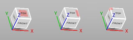
Figure 69 Navigation-cube controls (face, edge, vertex).

Table 7 Key combinations for switching viewpoints.

Viewpoint	Keyboard	Extended Numpad
Front	Ctrl + Shift + 1	1
Back	Ctrl + 1	Ctrl + 1
Right	Ctrl + Shift + 3	3
Left	Ctrl + 3	Ctrl + 3
Top	Ctrl + Shift + 7	7
Bottom	Ctrl + 7	Ctrl + 7

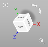
Figure 70 Navigation cube and arc arrows.

The Home command of the View menu or H keystroke restores the view to its original position.

The Fit to view menu option, button or F keystroke automatically fits the object to the 3D View window.

For point-clouds, you can have a look at scan from the Ray perspective. Open the right-click menu for this scan and select the Go to scanner viewpoint command to this end.

Displaying 3D Data

The toolbar on the right of the 3D View window features controls for data-display modes. If minimized, it can be opened by clicking button in the 3D View window (see Figure 70). All the commands for viewing and switching between modes are also available in the View menu.

Rendering and Shading Modes

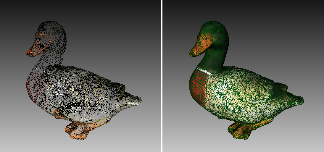
Figure 71 Examples of model using different rendering modes.

Point model on left and wire over solid on right.

Both the View menu and the 3D View toolbar allow you to choose one of the following 3D rendering options for scanned frames:

Render solid

the most common way to render with a solid fill on all faces using your selected shading method

Render wireframe

display polygonal-mesh edges without applying a solid fill to the faces

Render points

display polygonal-mesh vertices

Render wireframe over solid

apply a solid fill to the faces and use a different color to display edges. This method enables you to visually assess the quality of the polygonal model (see Mesh Simplification for details).

Render points and solid

automatically display scans in point view, but display models in solid-fill view. This mode eliminates the need to switch to another mode in order to find the best rendering approach for each surface type. It is enabled by default for the Artec Spider scanner.

For some examples of the various model-rendering modes, see Figure 71.

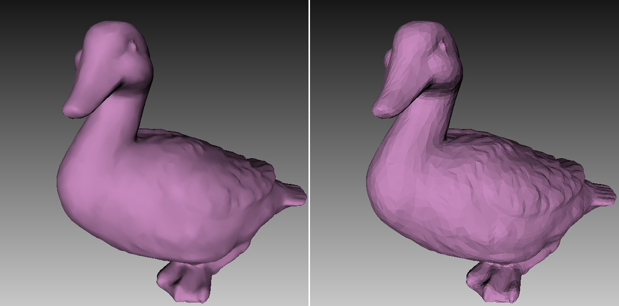
Figure 72 Smooth versus flat shading (respectively).

To choose a shading method for the solid fill, use the View menu:

Smooth shading

the color value for each point in a triangular face is calculated using color interpolation at the vertices

Flat shading

all the points on a triangular face are assigned the same color

Lighting, Color and Texture

The Lighting option in the View menu or in the toolbar, or L hot key toggles the lighting in the 3D View window. This option may be useful when you must turn the lighting off to see only the outline of the model or to assess texture quality.

The Color subgroup in the View menu or Color mode section in the toolbar list the methods for assigning colors to the surfaces in the 3D View window:

Texture	displays textured data; otherwise, the software uses the scan’s default color		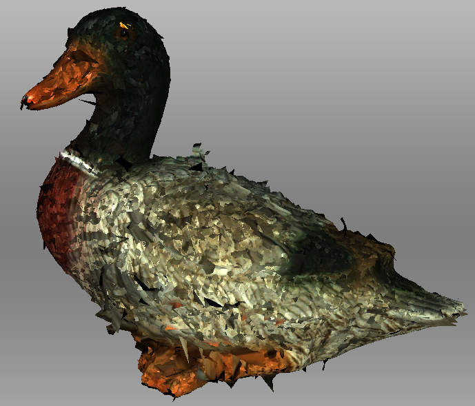Ctrl+Alt+1
Scan color	displays the default color of the scan; the figure depicts two scans		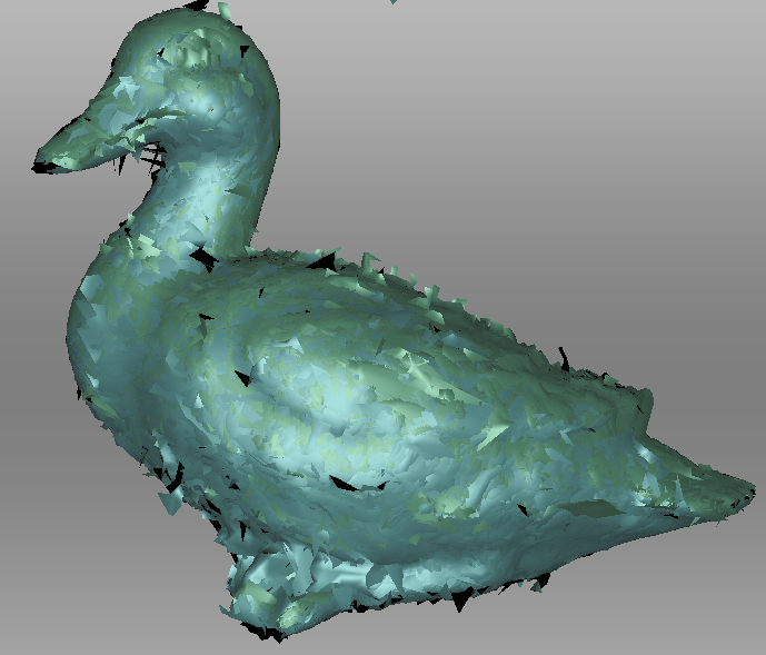Ctrl+Alt+2
Surface color	displays each frame in a scan using a different color		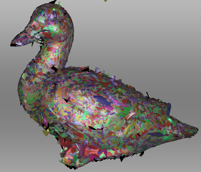Ctrl+Alt+3
Max error	colors the frames from Eva and Spider in accordance with their registration quality from green to red via yellow and orange; red indicates unacceptable values and registration errors		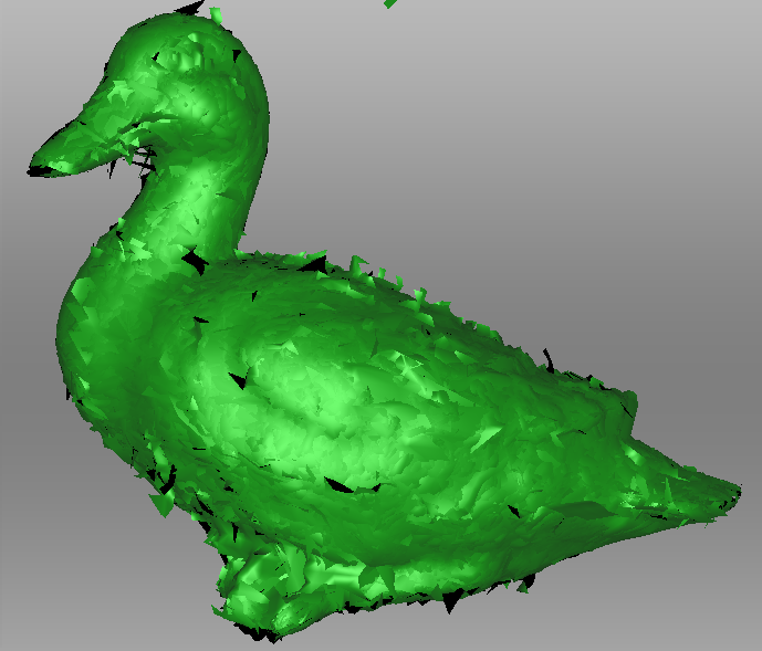Ctrl+Alt+4
X-ray	beneficial for noisy data since it highlights only areas with high point density; it features a slider for adjusting its intensity		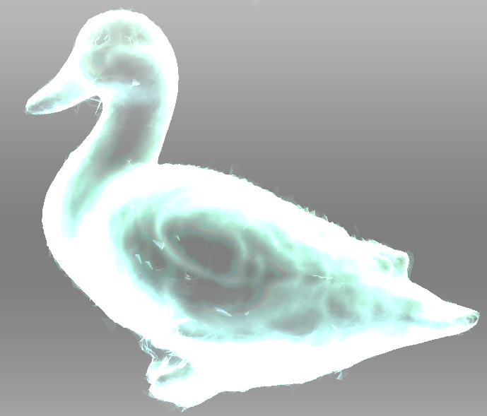Ctrl+Alt+5

Back-Face Rendering

Artec Studio offers three methods for rendering a frame’s back face:

Show

assigns the back face the same color as the model

Cull

the back face is not displayed

Black

renders the back face in black

You can choose the mode from the View menu or from the toolbar in 3D View window. See Figure 73 for examples that illustrate the different methods of back-face rendering. Black is the default mode.

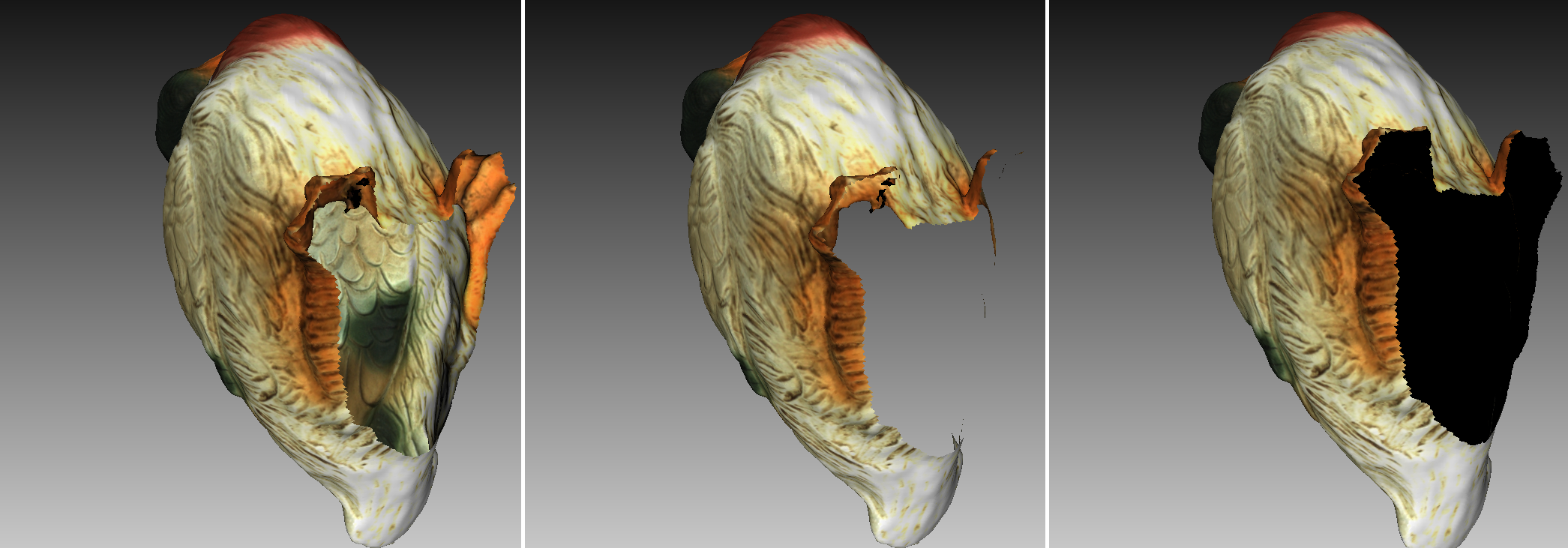
Figure 73 Examples of different methods for back-face rendering.

Show back-face mode on the left, hide (Cull) in the middle and Black on the right.

Representation of Normals and Boundaries

The Show normals option in the View menu enables or disables rendering of normals for each vertex. By default, the normals point away from the model surface and toward the 3D scanner. You can change this direction using the Invert normals command. You can also switch between modes for displaying normals by hitting the N key with the 3D View window active.

When working with edges, the Show boundary feature in the View menu allows you to enable and disable highlighting of the model’s edges. To toggle this feature, hit the B key with the 3D View window active.

Rendering and Texturing Untextured Polygons

Textured models may have some untextured areas (for instance, the green area in the middle of Table 8). The Render polygons without texture option in the View menu allows you to toggle rendering of such areas.

If the texture of the imported model is smaller than the model itself, Artec Studio can wrap it to fill the untextured areas (see Table 8). The wrapping effect is similar to floor tiling or a repeating wallpaper pattern—that is, the texture repeats periodically. To activate this option, enable the Wrap texture coordinates option in the View menu.

Table 8 Rendering and texturing untextured polygons.

Options Enabled	Result
None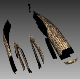
Render polygons without texture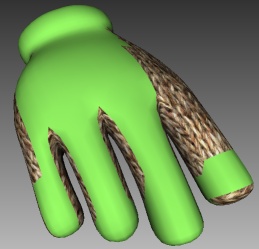
Wrap texture coordinates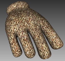

Displaying Boundaries of Texture Atlas

Textures applied to 3D models are obviously two-dimensional. You may, however, want to see the boundaries of each texture patch on the actual 3D surface. Artec Studio can display a texture-atlas file, such as the the middle image in Figure 118, with its boundaries highlighted (see Figure 74). Identifying the way in which the boundaries lie on the surface may, for example, help you determine whether you must simplify the model to get better texture application.

To enable boundary display, access the View menu and select Show texture boundaries or hit the Shift+B keys with the 3D View window active. To disable this feature, make sure this menu command is unchecked.

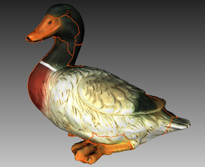
Figure 74 3D model with texture-atlas boundaries.

Technically, this command also works for textures produced by triangle methods, but it provides no usable information.

Saving Screenshots

You can capture surfaces displayed in the 3D View window and save them in a graphics file. Unlike the conventional system Print Screen command, this option saves only the contents of the 3D View window and uses the specified background color (see Background for screenshots transparent, black or white).

Tip

When saving screenshots in X-ray mode, avoid using transparent background.

To capture a screenshot, follow this procedure:

1. Select the Save screenshot… option in the View menu, or hit Shift+Ctrl+S.
2. In the dialog, specify the destination folder and file name, then click the Save button. Artec Studio will save the file in PNG format.

Note

If you save a screenshot using an existing file name, Artec Studio will overwrite that file without warning. Be sure to specify a unique file name to avoid overwriting other files.