Data Processing

Once you have captured an object from all desired angles and created a sufficient number of scans, you can then build a 3D model. This chapter offers a detailed description of the process.

See also

3D Scanning at a Glance.

• Reconstructing HD scans from saved raw HD data

• Revising Scans and Editing Scans

• Alignment

• Global Registration

• Creating Models (Fusion)

• Editing Models

• Texturing

Maximum Error and Registration Quality

Error is the parameter that reflects frame registration quality. For scans, it shows the maximum value among all the frames. The larger the value, the less accurate the alignment. Artec Studio displays noteworthy values only for scans that have passed Fine registration, Align and Global registration.

Table 9 Maximum error values for the scanner types.

	Good results	Acceptable	Unacceptable
Spider	0.0–0.1	0.2–0.3	0.4–…
Eva	0–0.3	0.4–0.9	1.0–…
Micro	0.0	0.1	0.2–…
Leo	0.0–0.5	0.6–1.3	1.4–…
Ray	0.1–0.9	1.0–2.9	3.0–…

Table 10 Other possible errors.

Error	Recommendations
Warning!	Check the frame list
Failed	Indicates unregistered frames in Show all frames mode

Reconstructing HD scans from saved raw HD data

If your scanner supports the HD mode (such as Artec EVA) and you used it to capture raw HD data without reconstructing HD scans (see Enabling HD Mode for details), then before you start building a 3D model, you may want to get HD scans from this data.

To launch the reconstruction of HD scans from your saved raw HD data, follow these steps:

1. In the Workspace panel, select one or more raw data scans (Figure 76, right).

   Note

   Raw data scans are not rendered in the 3D View window.

2. Open the Tools panel and locate the Raw data section (Figure 76, left).

3. Select the desired values for the HD-frames frequency and HD-data density parameters. For their description and setup recommendations, see Launching HD reconstruction after scanning.

4. Click Apply.

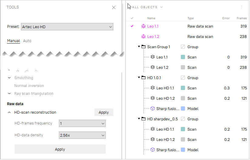
Figure 76 Launching HD scans reconstruction from saved raw HD data.

The Raw data section in the Tools panel on the left, a raw data scan selected in the Workspace panel on the right.

Important

The HD reconstruction is a time-consuming and resource-intensive operation. On slow computers, it can take up to several hours. If Artec Studio evaluates your computer’s resources as insufficient for the selected values of HD data density and HD-frames frequency, then the corresponding warning will be displayed. For information on resources requirements, see the Using HD mode section in System Requirements.

The HD reconstruction will start, and the corresponding progress bar will be displayed on the Status bar.

When the processing is complete, HD scans will appear in the Workspace panel. Their names will be marked with the letters “HD”, for example: Eva HD Scan 1.

Revising Scans

As you begin building a 3D model, you may want to start by preprocessing your scans: separate misaligned areas (if any) into separate scans and cut out unwanted objects from the scene.

You may encounter the following problems:

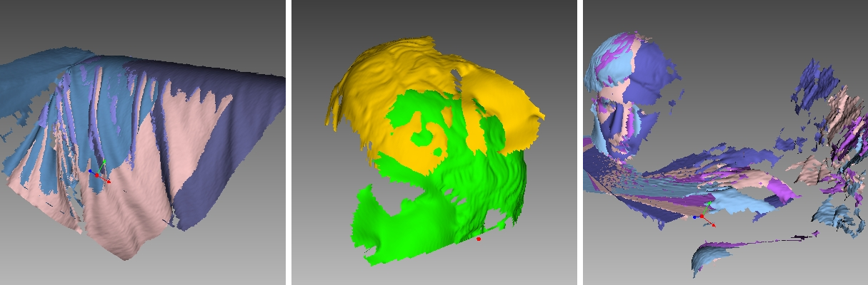
Figure 77 Possible scan errors.

Bad geometry on the left, scan misalignment in the middle and hands captured in frames on the right.

• Misaligned frames (see Figure 77, left)—may occur because of small size, an insufficient number of geometrical features on the object or an insufficient number of polygons in a frame.

• Misaligned parts (see Figure 77, middle)—occurs when the real-time alignment algorithm incorrectly determines the position of the new frame relative to previous ones.

• Unwanted objects in the frame (see Figure 77, right).

A visual inspection of the frames can be very helpful in determining problematic areas. To perform a visual inspection, select the scan and view all the frames that it contains by holding ↑ or ↓ on the keyboard. This technique can easily detect misaligned frames.

When viewing scans, application generally shows only key frames and textured frames. To display all the frames, select the Show all frames option in the 3D toolbar.

See also

Misalignment Detection.

Separating Scans

During the fine-alignment process, frames in certain scans may be misaligned. Sometimes it’s possible to divide the problematic scan into several scans, where each part is registered fairly well. In this case, divide the scan. To move some of the frames into a new scan, use the following procedure:

1. Select in the Surface List panel the frames you want to move (see Selecting Frames).

2. Click RMB and select Move to new scan (Figure 57, right).

You can also fix alignment errors in another way: reset the current frame-transformation values and repeat the registration, making any appropriate changes to the settings. Select the desired scan in the Workspace panel, click on it using RMB and select Unregister from the dropdown menu. Doing so will reset the computed positions of individual frames in the scan. A dialog will then appear, prompting you to confirm the operation. To compute new positions, run the Rough serial registration and then Fine registration algorithms (see Fine Registration).

Alignment and Registration at a Glance

Registration and alignment tools perform similar tasks, however, they differ. Use the table below to get an insight into the details.

Table 11 Understanding registration and alignment modes.

Type	Purpose	Details
Fine registration	Adjusting frames’ positions	Treat scans in batch separately. Starts once you leave Scan panel.
Align	Assembling scans	See also Table 12
Global registration	Optimizing frames within scans	Launch it for a pre-aligned batch of scans or for a single scan
Rough registration	Preliminary registration performed during scanning	No need to start it manually
Photo registration	Applying texture to models with registered photographs	See also Texturing

Editing Scans

To edit scans, open Editor from the side panel and select the Eraser tool. You can also use Positioning tool or Transformation tool to orient the scanned data.

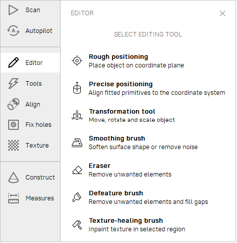
Figure 78 Editor panel.

Eliminating 3D Noise (Outlier Removal)

During the scanning process, so-called outliers may appear in the scene. Outliers are small surfaces unconnected to the main surfaces. They require removal because they may spoil the model or produce unwanted fragments. Artec Studio provides two ways to remove outliers: erase them before fusion (preventive approach) or after fusion (“furthering” approach—see Small-Object Filter). We advise using the former approach because it decreases the possibility of improper fusion by preventing noisy features from attaching to the main surface.

This outlier-removal approach is based on a statistical algorithm that calculates for every surface point the mean distances between that point and a certain number of neighboring points, as well as the standard deviation of these distances. All points whose mean distances are greater than an interval defined by the global-distances mean and standard deviation are then classified as outliers and removed from the scene.

For better results, we recommend running global registration before starting the algorithm. If you begin Outlier removal before doing so, a dialog will appear prompting you to perform global registration.

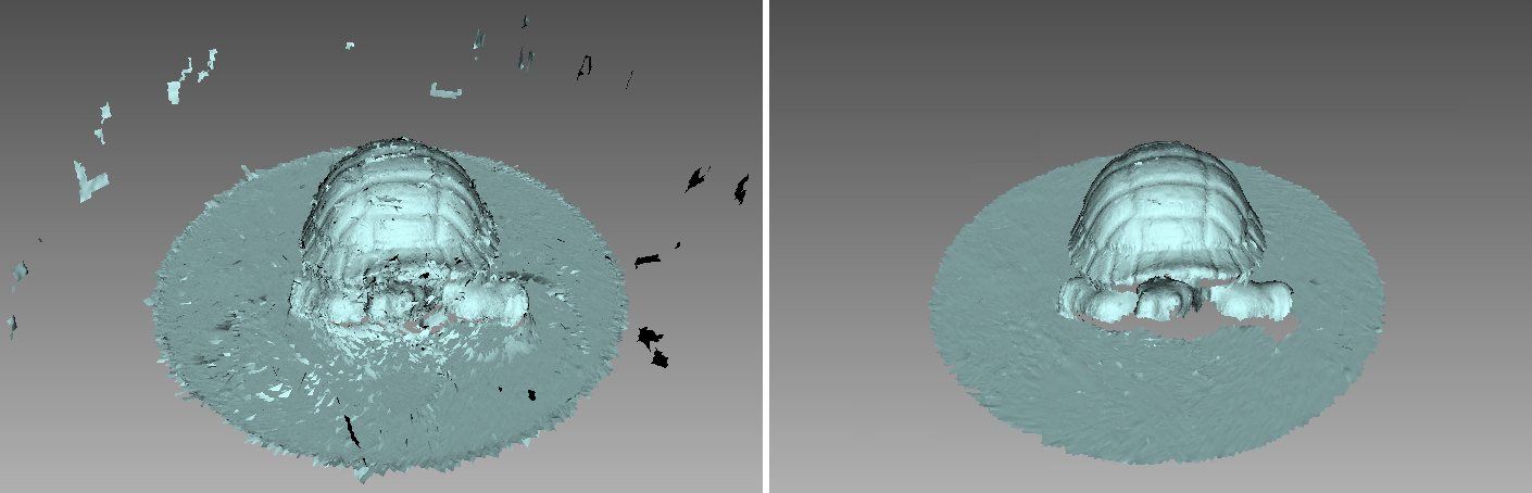
Figure 79 Outlier removal: before and after.

In most cases, none of the parameters accessible through the button requires adjustment. But if necessary, you can change the values of these parameters:

• 3D-noise level is a standard-deviation multiplier. We recommend choosing the value for this parameter according to the following guidelines:

  • 2 for noisier surfaces

  • 3 for less noisy surfaces

• 3D resolution, mm should be set equal to the resolution of the Fusion process that you expect to run later.

Click Apply to run Outlier removal.

Erasing Portions of Scans (Eraser)

Nearly always, the scanning process will capture unwanted elements, such as walls, the operator’s hands, surfaces on which the object is located and other extraneous objects. This unwanted data can hinder postprocessing. To avoid this problem, we recommend eliminating these objects before processing. Eraser offers several options to quickly and easily remove unwanted elements from the scene (see Selection Types).

1. Open the Editor panel using the side toolbar.

2. Open the Eraser tool by clicking or by hitting E.

3. Select one or more scans in the Workspace panel.

4. In the Editor panel, choose the required selection type.

5. Consult the instructions for a specific mode and select regions on the scans that you want to erase. To clear all selections, click Deselect.

6. Click Erase to eliminate the area highlighted in red or to apply cutting plane (Cutoff-plane or Base selections).

To undo changes, click in the Workspace panel or menu Edit, or hit Ctrl + Z. Each click of the Erase button generates a command history entry. To undo several operations, use the dropdown menu of button and select the lowest entry.

Selection Types

Type	Illustration	Usage
2D		Hold down Ctrl and use Scroll wheel to adjust the tool size. Paint with Ctrl+LMB to create a selection.
3D		See above.
Rectangular		Use Ctrl+LMB to select a rectangular region.
Lasso		Use Ctrl+LMB to freely outline an irregular region. You can release LMB (not Ctrl) and then continue clicking on desired points to select a desired shape.
Cutoff-plane		Create selection as in 2D mode. Once you have released the mouse button, a plane will appear. If necessary, adjust the plane level by using Scroll wheel while holding down Ctrl+Shift or orient the plane freely in 3D space. To this end, hit Alt to display the designated control. Then still holding the key, drag the required control ring.
Base		Select a flat area as in 2D mode. The tool will automatically fit the base plane and select everything below it.

If the Select through checkbox is selected, all surfaces throughout the scan are affected. If not, the brush only works on the visible surface.

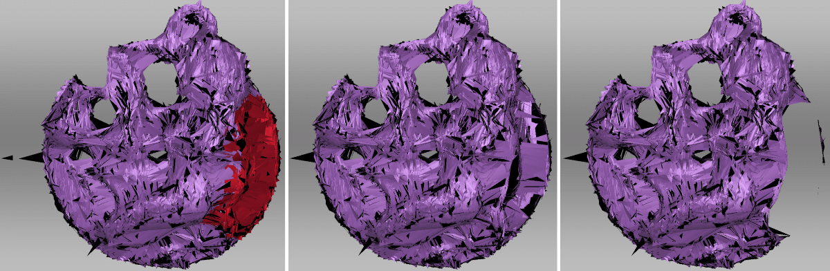
Figure 80 Select through in 2D selection: disabled in the middle, enabled on the right.

Use the following general procedure to erase unwanted elements:

See also

Hot keys in Editor.

More Actions With Selections

Apart from erasure, you can perform the following action with the selected regions:

• Clear selection to create a new one. Click Deselect or reselect the region manually while holding down Ctrl+Alt.

• Invert selection (clear the highlighted region and select the rest). It might be useful when working with large scans. Click Inverse or hit I.

• Temporarily hide selection if it obstructs the region you want to erase. Click Hide to this end. To display hidden polygons, click Show. Then select the region you want to erase.

Erasing Supporting Surface

Artec Studio offers two selection modes that differ from conventional brushes in the way how you select the area for erasure. First, you indicate the flat surface (table, floor or base) on which the object is resting. Then, application either determines the base plane and select the area underneath it (Base selection, Figure 81), or creates a cutting plane (Cutoff-plane selection) that divides the scan into two parts: the first will remain and the second will be erased (see Figure 82). You can orient this plane in any way you need.

Tip

Consider using the Enable automatic base removal option when scanning since it deletes the flat surface automatically after you close the Scan panel.

Figure 81 Base selection in action: indicating a flat region → defined base → removed base.

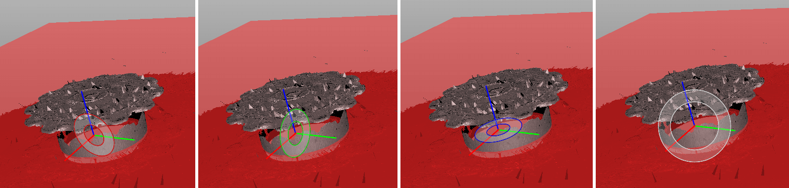
Figure 82 Various controls for orienting cutoff plane: around axes (X, Y and Z) and view direction.

Fine Registration

Fine registration is an algorithm designed to precisely align captured frames.

In a number of cases you can start the Fine registration algorithm manually using the Tools panel. To access a list of parameters, click the button in the Fine registration section. The algorithm affects all scans marked with the icon in the Workspace panel (see Selecting Scans and Models for more information on scan selection), but it processes them separately.

Features	Geometry and texture or Geometry	The type of algorithm that will perform scan registration. The former is preferable as it takes both geometry and texture into account. If your scan entirely lacks texture, we recommend using Geometry option.
Subsampling	0.01–1	The option makes the input geometry data less dense to speed up the processing. Use lower values for objects with poor geometry. Designed for scans with HD reconstruction, this option can speed up processing in Geometry and texture mode.

Alignment

Although Artec Studio features continuous scanning, there may be some cases where the application lack sufficient information about the relative positions of multiple scans. To assemble all scans into a single whole, you must convert the data to a single coordinate system—that is, you must perform alignment using the Align tool.

Hint

First refer to Auto-Alignment and take a glance at the Summary of Alignment Modes section as well.

Selecting Objects for Alignment

In the Workspace panel, use the flag to mark all scans or groups that you intend to work with. Once you click Align in the side panel, the marked scans and groups will appear in the left panel already selected in the same order as they appear in the Workspace panel.

Note

Workspace group of scans is treated as a single entity. To release objects constituting the group, use the Ungroup item from the dropdown menu.

During the Align operation, Artec Studio divides the selected scans or groups into two collections: registered (aligned) and unregistered (unaligned). The first collection initially contains only one scan (the first one in the list) or group, which are highlighted in blue. Collection name appears in bold and uses the same color icon ( or ). Auto-Alignment, however, may produce several collections of aligned scans.

The user’s task is to align all scans to those that are already registered and to “assemble a model”. In general, the procedure includes the following steps:

1. Click the required tab in the Align panel.

2. Select one scan or group () from the unregistered collection in the Align panel. The name of unregistered scan appears in a regular typeface. When selected, the unregistered scan is marked by the green icon , whereas the group is marked by icon . You can select several scans using either of the following methods:

   • Press and hold down the Ctrl key, and then click each scan or group that you want to select

   • Click the first item, press and hold down the Shift key, and then click the last item.

3. If necessary, specify point pairs (for two scans) or sets of points (for more than two scans)

4. Click the desired alignment-command button (Auto-Alignment is the most recommended one). The command affects all scans selected in the Align panel plus the first one ().

Note

If other objects, except for scans, belong to a group, you can also position them simultaneously with the scans. Select the Apply to all objects in parent groups checkbox to this end.

Since each mode varies in its effects, see the details in the corresponding subsections for more information. Note that you can use either one mode or a series of modes (see comparison table in Summary of Alignment Modes): drag alignment, rigid alignment with and without point specification, automatic rigid alignment, and alignment with surface deformations.

Changing Object Status

If you have already aligned several scans, you should move them to the registered collection. Select them in the Align panel using LMB. Next, click RMB on the name of any scan and select the Mark as registered option from the dropdown menu, or just double-click its name in the list. At this point, Artec Studio will treat registered scans as one, so you cannot move them independently.

If you accidentally mark a scan as aligned, remove it from the registered collection by selecting the Mark as unregistered item from the dropdown menu, or just double-click it.

Displaying Objects in 3D View

Objects selected in the Align panel appear in the 3D View window. Keys 1, 2 and 3 switch among objects in the 3D View window:

1	Shows aligned scans, groups and collections
2	Shows scans and groups that are currently under alignment
3	Shows all scans and groups

Navigation in align mode is similar to navigation in the 3D View window:

Rotate	Hold LMB and move mouse
Zoom in/out	Scroll the Mouse wheel, or hold RMB and move mouse
Move freely	Hold LMB and RMB simultaneously, or hold the middle button, and move mouse

Summary of Alignment Modes

The table below provides basic information on the various alignment modes (see Alignment).

• Object type lists which scans and models you can use in a particular mode.

• Scans per operation is the number of scans required to use a particular mode.

• Markers in set prescribes how many markers (points) you can map in one point set. Some modes require point (marker) sets, but some don’t.

• “—” means that markers are unnecessary.

• “0 or 2” means point specification is optional and, if you do specify them, only marker pairs are allowed.

• “At least 1” means you can specify an unlimited number of markers in one set.

Table 12 Parameters for alignment modes.

Mode	Object Types	Objects per Operation	Markers in Set	Notes
Rigid (markers)	Any	2	2	Considers only coordinates, not geometry
Rigid (meshes)	Any	2	0 or 2	Considers geometric features
Rigid (texture)	Scans with poor geometry	2	0 or 2	High resource consumption
Rigid (auto)	Any	Any number	—	Works if surface is well textured
“Drag”	Any	2	—	Interactive
Nonrigid	Polygon models	Any number	0 or 2	Deforms surfaces and textures; pre-alignment required
Complex	Any	1 (at least 2 for models)	At least 1	Precise and flexible

Drag Alignment

Drag alignment is always available, regardless of which tab is active in the Align panel. This mode allows you to align scans by manually dragging them in the 3D View window.

Owing to the low accuracy of this approach, however, you can optionally use it for preliminary alignment before running more-accurate modes.

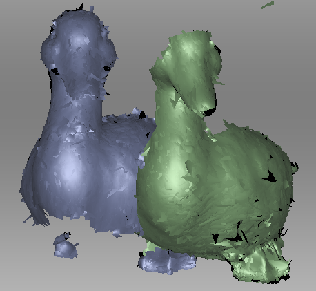
Figure 83 Dragging a scan

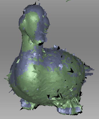
Figure 84 “Drag” alignment result

1. Select the scan you want to align, keeping in mind the recommendation in Selecting Objects for Alignment. Artec Studio allows you to select multiple scans, but note that it will align them with the registered scans as a single unit.

2. Holding down the Shift key and one mouse button, move and rotate the scan you’re aligning (a green one ) close to the registered scan (a blue one ). Here is a list of allowed movements and corresponding buttons:

   • Shift+LMB to rotate

   • Shift+LMB+RMB to move

   • Shift+RMB or Shift+Scroll to move only unregistered scan along the view direction

3. To confirm the alignment, release the mouse button(s) and the Shift key, then click Apply. Note carefully that any scans you are registering won’t automatically move to the registered set (see Figure 84). You can do so manually as the Changing Object Status describes.

4. If you have several scans to align, repeat these steps for each one individually.

Auto-Alignment

Rigid alignment is a universal mode suitable for aligning most scans. Auto-alignment is the easiest approach, however. The advantages of this latter mode include the ability to align several scans at once and avoid the need to specify points; the only disadvantage is minimum requirements for the size of the overlapping areas in the scans you’re aligning.

To perform auto-alignment, follow these steps:

1. Make sure the Best fit tab is selected in the Align panel (see Figure 85). The tool will automatically select all scans. Clear unnecessary selections by using the Ctrl key (see Alignment).

2. Click Auto-alignment. Ideally, Artec Studio aligns all the scans and marks them using the icon. It may, however, mark scans as registered even though the 3D surfaces failed to join properly.

Important

Auto-alignment may be unsuccessful if the scans have small overlapping area.

Auto-alignment may produce the following results:

• Aligned scans, marked with the icon (basic collection of registered scans)

• Unregistered scans, marked with the icon

• One collection () or several collections (, ) of registered scans. Scans forming this collection failed to align with the basic registered collection (), although they succeeded in aligning with each other.

We recommend resolving issues with unregistered scans or registered collections by aligning them manually as Manual Rigid Alignment with Points describes. Other methods may also help.

Managing Collections and Scans

You can perform the following actions on the scans from the list in the Align panel (right-click on the item to open the context menu):

• Mark as registered. Only available for single unregistered scans or groups ( → )

• Mark as unregistered. Use this command to discard the alignment state of a particular scan (unavailable for scans)

• Select collection highlights the respective collection (, , and so on)

• Mark collection as registered converts all scans from the collection into the basic registered collection ( → )

Manual Rigid Alignment Without Specifying Points

You can perform rigid alignment either with or without specifying points. If the scans are close to each other in distance (e.g., after “drag” alignment), or if they have a large overlapping area or rich texture, you can skip the task of point specification when aligning them.

Perform the following steps:

1. Make sure the Best fit tab is selected (see Figure 85).

2. Select the scan you want to align, as the beginning of Alignment describes.

3. Click Align. The result should be as Figure 87 depicts. If you are dissatisfied with this result, click and follow the recommendations in Manual Rigid Alignment with Points.

4. Select another scan from the list of unregistered scans and repeat the above procedure.

5. Click Apply to confirm your alignment results or Cancel to reject them.

Texture Alignment

If the object was scanned with texture, the texture-alignment feature may ease the alignment process. It uses texture-image characteristics of scanned objects and greatly decreases the possibility of incorrect alignment. This feature also helps to align objects with few or no geometrical features, such as round or flat objects with no corners. If an object has rich, nonrepetitive geometry, however, we recommend disabling texture alignment to reduce the algorithm’s running time. Also keep in mind that texture alignment will be useless if the object texture is monochrome.

To enable texture alignment, select the Enable texture alignment checkbox at the bottom of the Align panel just before you perform Step 3 of the procedure above.

Note

Texture alignment is a resource-intensive algorithm that slows down the alignment process. We recommend using it only in cases where the object’s geometrical features are insufficient.

Specifying Points and Editing Their Positions

Before considering how to align scans using points, it is helpful to highlight point-pair specification. The alignment algorithm uses pairs of point, or point sets in Complex alignment mode (Complex Alignment), to detect scan areas that should be brought close together.

To do point alignment, create several point pairs. To create one pair, mark one point on the aligned scan and then mark another one on the unaligned scan. Ensure that in each case the points for a given pair match a corresponding point on the surface of a real object; note, however, that high matching accuracy is unnecessary, since Artec Studio only uses the pairs to gain a rough approximation before performing precise registration. In the Complex mode, you can create a set of points (instead of just a pair), i.e. you can simultaneously specify more than two points in one or several unregistered scans and only one in the registered scan. All these points are connected by polylines and form a set.

When specifying points in the Rigid and Nonrigid modes, the application automatically creates pairs. Having specified one pair, you can immediately create the next one. In Complex mode you must confirm set creation by hitting Space or by clicking New set from the left panel, because the set may comprise multiple points (see Figure 86 and Figure 92).

You can toggle between the point pairs (sets) by hitting Space and Backspace, or by clicking RMB in the 3D View window and selecting the relevant options from the menu. You can also relocate points in the pair (set). Hover the mouse cursor over the point until the pair (set) is highlighted in white, then drag the point to the proper position using LMB, or select the pair (set) and specify a new position using LMB. To confirm your actions and deselect the pair (set), hit Space. You can also remove either a pair (set) or one of its individual points: click on the point using RMB and choose the appropriate command from the menu. Alternatively, you can use Del to remove the selected pair (set).

Manual Rigid Alignment with Points

We advise using this mode for scans located at a significant distance from each other or when aligning polygon models with CAD models.

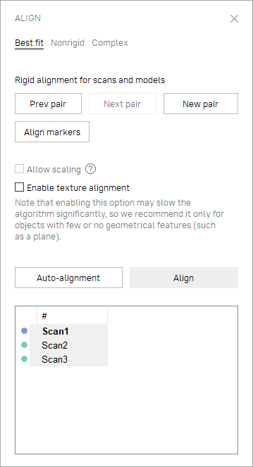
Figure 85 Align panel: Best fit tab.

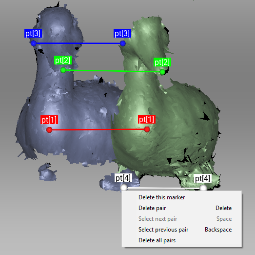
Figure 86 Creation of point pair.

Figure 87 Alignment result.

To use this approach, follow these steps:

1. Make sure the Best fit tab is selected (see Figure 85).

2. Select the object you want to align, as the beginning of Alignment describes.

3. Specify several point pairs (Figure 86), keeping in mind the recommendations from Specifying Points and Editing Their Positions.

4. Click Align markers. This mode takes into account only the coordinates of specified points and tries to reduce the distance between the markers for each pair.

5. Carry out Steps 3–5 of the procedure in Manual Rigid Alignment Without Specifying Points.

Nonrigid Alignment

Whereas rigid alignment can only perform such transformations as translation and rotation, the nonrigid algorithm can deform 3D data. This algorithm is intended to process so-called nonrigid objects: objects whose shapes have changed during the scan (e.g., models of animals or humans—see Figure 89, left). Keep in mind that the surface Artec Studio produces as a result of the deformation may differ from the surface of the actual object.

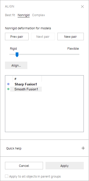
Figure 88 Align panel: Nonrigid tab.

Figure 89 Two models after rigid (left) and nonrigid alignment (right).

Note

Nonrigid alignment works on models only. Thus, before you run it, prepare models by fusing the source scans. It is also necessary to first align models in rigid mode (see Manual Rigid Alignment Without Specifying Points, Auto-Alignment or Manual Rigid Alignment with Points).

To run the nonrigid alignment, follow these steps:

1. Make sure the Nonrigid tab is selected (see Figure 88).

2. Select the models you want to align, as the beginning of Alignment describes.

3. If the models differ significantly from each other, we suggest that you specify several point pairs, keeping in mind the recommendations in Specifying Points and Editing Their Positions.

4. Where necessary, adjust the deformation degree using the flexibility slider. The greater the flexibility value (i.e., the more “flexible” the deformation), the longer the computation will take.

   Warning

   Avoid extreme Flexibility values. Applying very large values may result in major surface distortions and may slow down the algorithm. Extremely low values, on the other hand, barely deform surface and often fail to produce the expected nonrigid-alignment results.

5. Click Align…. The algorithm will align models by deforming one of the model (see Figure 89, right). If you are dissatisfied with the alignment results, click and specify additional point pairs, or reposition the current pairs.

6. Select another model from the unregistered set and repeat the steps above.

7. Click Apply to confirm your alignment results or Cancel to reject them.

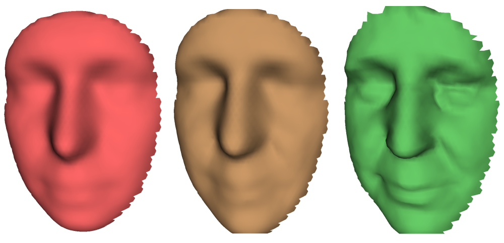
Figure 90 Flexibility slider in action: original model (left), nonrigidly aligned model with low Flexibility value (middle) and with high value (right).

Note

This version of Artec Studio does not support texture mapping on nonrigidly aligned models.

Complex Alignment

Complex alignment allows you to align not only scan to scan, but surface to surface within a given scan (see the mode comparison in Summary of Alignment Modes). Relative to other modes, this one supports multipoint-set definition—that is, you can link more than two points. It’s useful for aligning scans obtained during circular movements of the 3D scanner in cases where fine or global registration fails to align them. To run the Complex alignment, perform the following steps:

Figure 91 Align panel: Complex tab.

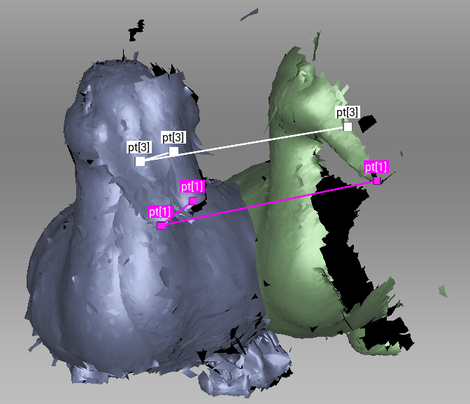
Figure 92 Before alignment: two point-set added.

Figure 93 Alignment result.

1. Make sure the Complex tab is selected (see Figure 91).

2. Select the scans you want to align, as the beginning of Alignment describes. This mode allows you to work even with just one registered () scan.

3. Specify one or more point sets on the scan surface (see Figure 92), keeping in mind the recommendations in Specifying Points and Editing Their Positions.

4. Click Align… to run the alignment with your specified restrictions (Figure 93 shows example results). If you are dissatisfied with the alignment results, click and specify additional point sets, or reposition the current sets. To redo an operation that you have undone, click .

5. Click Apply to confirm your alignment results or Cancel to reject them.

Global Registration

Once you have aligned all your scans, proceed to the next stage: global registration. The global-registration algorithm converts all one-frame surfaces to a single coordinate system using information on the mutual position of each surface pair. To do so, it selects a set of special geometry points on each frame, followed by a search for pair matches between points on different frames. To perform correctly, the algorithm requires an initial approximation, which a user ensures in the course of the Align operation.

Note

Global registration is a resource-intensive operation. Processing of large data sets may take a long time and require a large amount of RAM.

Before launching the global-registration algorithm, you can fix the position of some of the scans and/or their frames if necessary (for detail, see Locking Object’s Reposition).

To launch the algorithm,

1. Select all aligned scans in the Workspace panel.

2. Open the Tools panel.

3. Locate the Global registration section.

4. Check the Preset field. It must display the actual scanner that was used to obtain the selected scans.

5. Click Apply.

Global-Registration Parameters

Features	Geometry and texture or Geometry	The type of algorithm that will perform scan registration. If an object has rich texture and poor geometry, consider using the Geometry and texture option. For objects with rich geometry, you can choose Geometry mode to increase the registration speed.
Registration mode	Separate or Collective	This enables registration of selected scans separately (one by one), altogether collectively, or both separately then collectively. Does not work with the Artec Ray preset.
Focus on geometry	On/Off	Enable it for objects with rich geometry and poor texture. In comparison with Geometry mode, it also considers texture. If enabled, this option skips checking quality of geometry registration, taking the rich geometry for granted. It is only available for Geometry and Texture mode.
Key frame ratio	0–0.6	Determines how many surfaces are treated as key frames. Decreasing this parameter when processing a feature-rich object may speed up registration. Increase it if only the previous attempts to register scans failed. Technically, values higher than 0.7, including 1, are possible, but they may significantly slow down the algorithm.
Search features within, mm	3–5 mm (Spider); 5 mm (Eva/Leo) and 50 mm in Geometry and texture mode	To align frames, the algorithm needs information on how far away the identical features are distributed on the adjacent frames. Lower this search radius for objects with many repetitive features and increase for large objects to ensure the algorithm robustness. Increase this parameter sparingly since large values may cause erroneous registration and hinder calculation. Adjust it if Fine Registration completes with inappropriate values of maximum errors.
Smart subsampling	On/Off	Enable it to allow Artec Studio to automatically adjust the input geometry data as required, to speed up the processing. Designed for scans with HD reconstruction, enabling this option can speed up processing in Geometry and texture mode.

Locking Object’s Reposition

When you perform operations that change the relative position of objects (such as Global Registration), it may be necessary sometimes to lock the repositioning of some of these objects. Consider, for example, the case where you work with several scans made in the Target-Assisted Scanning mode. The initial relative position of such scans in space should be preserved.

Artec Studio supports two types of locking mechanism:

• Lock registration () - locks the repositioning of scan frames relative to each other during the global registration but allows you to move the scan itself. This mechanism applies only to scans containing frames, that is, obtained using handheld scanners such as Artec EVA, Spider, Leo, or Micro.

• Lock position () - locks the repositioning of the object relative to the global coordinate system. This mechanism applies to scans and any other objects.

Note

Lock registration is the same mechanism that was called Lock in Artec Studio 15 and earlier.

The Lock position status affects not only the results of global registration but also the operations of Positioning and Transformation tools (see Preparing Models To Export for details). When using these tools, any reposition of objects with the Lock position status is blocked.

You can lock or unlock a specific object in the Workspace panel:

• using the context menu of this object, or

• by clicking the object row in the Lock column area ()

To lock or unlock all objects in the Workspace panel, click the header of the Lock column ().

To lock or unlock all objects in a group, click the group row in the Lock column area ().

Note

When you change the lock status of several objects at once, the result of the mouse click will depend on the types of objects that are displayed in the Workspace panel or included into the group and on the current lock status of these objects.

Global Registration for Point-Cloud Scans

Global registration with the Artec Ray preset only runs on several point-cloud scans. Artec Studio offers four modes:

• Targets considers only targets (spheres and checkerboard targets)

• Geometry Ray. The prerequisite step for this mode is alignment. The scans must have sufficient initial approximations and may not have targets.

  • Search features within, mm defaults to 150 mm.

• Targets and geometry. Global registration first runs on the basis of targets, then on geometric features.

• No targets (Geometry alignment) is suitable for point-cloud scans captured without targets. It doesn’t require alignment, but you need to run Geometry Ray afterwards.

  • Distance from scanner, mm is a radius around the scanner viewpoint from where the algorithm will take points. Alter it when you need to ignore the background 3D noise.

  • Feature voxel, mm is a volume measure to cull extra points from the algorithm input. The more the value, the more the points will be culled and the faster the algorithm. Increase it sparingly since it affects the algorithm accuracy.

  • 3D-noise level, (0.01-0.02) is a factor to adjust the point culling. Increase it for point-cloud scans with noisy areas. Decreasing it will result in increasing the algorithm robustness and duration. The recommended range is 0.01–0.02.

Possible Global-Registration Errors

• After the global-registration algorithm finishes, the frames are in disarray (see Figure 94, left) or the frame positions are unchanged. This error occurs because the application is configured for a different scanner type than the one that captured the data. Change the device type in the application settings (see Algorithm Settings).

• The algorithm has completed successfully, but a gap exists between two or more scans (see Figure 94, right). Select just these scans in the Workspace panel and run the global-registration algorithm. If the scans have drawn closer to each other but have failed to align after the algorithm finishes, increase the number of iterations and rerun the algorithm. Repeat this process until you achieve full alignment, then run global registration once again for all data. If you are unable to align several problematic scans, try aligning just two of them, then gradually increase the number of scans until all of them are aligned.

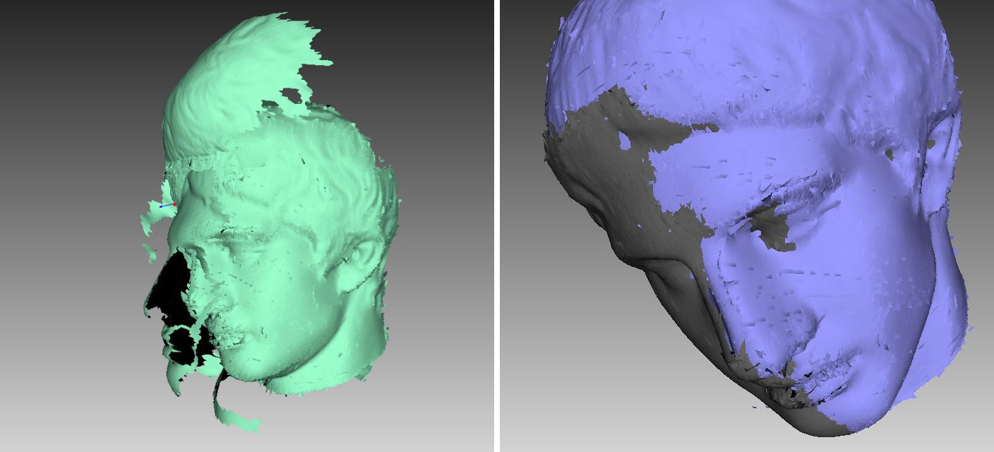
Figure 94 Global-registration errors: wrong settings on left and gap between scans on right.

Transferring Transformations

Sometimes it can be useful to transfer transformations from one scan to another (see Use Cases for Transformations Transferring). The transfer of transformations means that all transformations of scan frames resulting from the application of different Artec Studio tools are sequentially repeated for all frames of another scan. The transformations of the source scan as a whole are copied to the destination scan as well, including the global registration status.

Note

In general, you can transfer transformations from one scan to any other scan. However, of practical interest are only the cases when the source and destination scans are copies of each other.

To transfer the transformations from one scan to another, perform the following actions:

1. In the Workspace panel, right-click the source scan and choose Copy Transformation from the context menu (see Figure 95, left). The transformations of the source scan and its frames will be saved.

2. Select one or several destination scans.

3. Right-click the selected scan(s) and from the context menu choose Paste from <source scan name> (see Figure 95, right).

All saved transformations will be sequentially applied to the selected scans and their frames. After the transfer is finished, the information about the saved transformations will be erased.

You can use the corresponding buttons of the main window to undo and redo the transfer of transformations (see History of Project Changes).

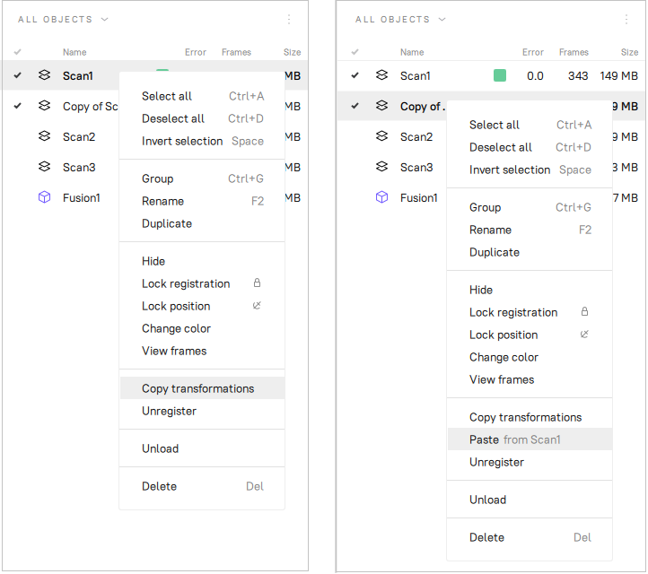
Figure 95 Transferring transformations: copying transformations (left) and pasting them (right)

Use Cases for Transformations Transferring

Use case 1: Saving time when processing HD scans

Global registration of HD scans is a very time-consuming operation: several times longer than it takes for SD scans. To save time, you can utilize the following scheme:

1. Make a copy of an HD scan.

2. Treating the scan copy as an SD scan, perform all the required transformations including the global registration.

3. Transfer the transformations from the copy to the original HD scan.

Use case 2. Saving time when working with backup copies of scans

Global registration takes longer than any other scan and frames transformation. Therefore, replacing the Global registration with the transformations transfer may save time.

Consider the following scenario:

1. You make backup copies of scans and then only work with the original scans.

2. You remove some excess parts of the scans using Eraser, run Global registration, apply Outlier removal and finally perform the Fusion operation.

3. After examining the resulting model, you conclude that you removed too much when working with the Eraser and/or the Outlier removal.

You have to undo all previous operations and once again repeat the sequence of actions, including Global registration. To avoid the latter and save time, you can instead transfer the transformations from the current scans to their backups and then continue working with the backups.

Ray Scan Triangulation

Application offers two ways to convert point-cloud surfaces to the commonly used models:

• Fusion operation

• Special triangulation algorithm

The latter approach is preferable to fusion in terms of speed. It generates a polygonal mesh from the original point cloud by simplifying its structure.

To launch this algorithm, follow the steps:

1. Mark a scan from Artec Ray using flag in the Workspace panel.

2. Access Tools from the left toolbar.

3. If necessary, specify the Decimation ratio and set either of the threshold filters.

4. Click Apply.

Mode	Simple, Adaptive (distance-aware)	Adaptive takes into account the distance from the scanner, whereas Simple removes points with the fixed step (Decimation ratio)
Decimation ratio	1–10	The larger the value, the more the points will be culled. 1 leaves the point cloud unchanged. 2 culls half of the points, 4 keeps some 25% of the total amount of points, 10 about 10%.
Stitch sections	On/Off	Enable it to stitch sections of the point-cloud scans
Render mesh based on	Vertex colors, Distinct colors for sections, One random color	It can color an output model on the basis of Vertex colors or sections constituting the point-cloud scan. The latter yields multicolor model.
Desired edge length, mm		Adaptive (distance-aware) method tries to maintain this edge length for triangles within the entire model.
Polygon edge length (max), mm	Above 0.1 mm 1	Algorithm will remove triangles whose edge lengths are greater than the specified value.
Polygon angle (min), deg	1–60 1	Triangles with angles smaller than specified limit (in degrees) won’t be created in the resulting mesh. Extremely large values that are out of the recommended range may yield no mesh.
Incidence angle (max), deg	0.1–90 1	If the angle between the normal to triangle and the scanner view direction is larger than the specified one, this triangle is subject to removal.
Incidence angle between vertices (max), deg	0.1–90 1	The algorithm will remove triangles whose edges form angles (toward the scanner viewpoint) greater than the specified limit (in degrees).

1(1,2,3,4)

Use 0 value to disable a particular filter.

Creating Models (Fusion)

Fusion is a process that creates a polygonal 3D model. It effectively melts and solidifies the captured and processed frames. Fusion is the most interesting part of the processing task because a polygonal 3D model is what most people expect to see when performing a 3D scan. To this end, you can use one of the following algorithms, each of which has a self-explanatory name (see also the summary in Table 13):

• Fast fusion produces quick results.

• Smooth fusion is good for scanning the human body because of its ability to compensate for slight movements by the person you’re scanning.

• Sharp fusion perfectly reconstructs fine features and is suited to both industrial objects and human bodies. It is the only mode that allows you to use all the capabilities of a Artec Spider scanner.

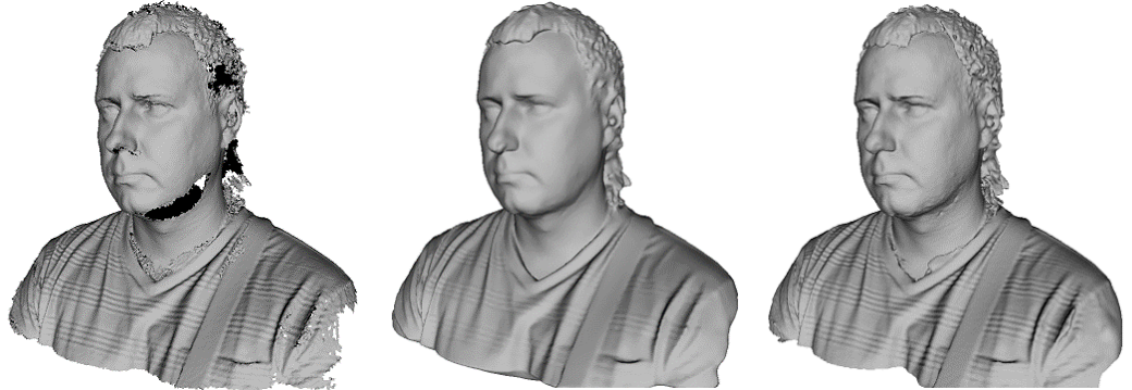
Figure 96 Models of a human subject obtained using various algorithms: Fast fusion (left), Smooth fusion (middle) and Sharp fusion (right).

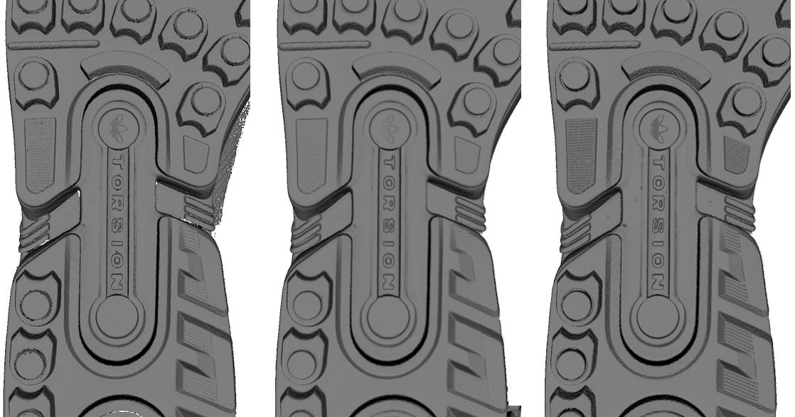
Figure 97 Models of a shoe sole obtained using various algorithms: Fast fusion (left), Smooth fusion (middle) and Sharp fusion (right).

Table 13 Comparison of fusion modes.

	Fast Fusion	Smooth Fusion	Sharp Fusion
Usage	Fast results for large data sets; also for measurements	Large, noisy data sets with patchy missing regions; scans of moving objects	Scans from Artec Spider; scans having regions with fine details and sharp edges
EVA	resolution no less than 0.5
Spider	resolution no less than 0.15
Leo	resolution no less than 0.6
Fill holes	Not applicable	Available
Features	Resulting surfaces are relatively noisy.	Smoother results. Can compensate for slight movements, but not recommended for accurate measurements. Relatively slow.	Higher level of detail. Faster than Smooth fusion, but may intensify existing noise.

To obtain a model:

1. Make sure the scans you intend to fuse have passed Global registration.

2. Select the scans in the Workspace panel using .

3. Enter the Tools panel.

4. Select the necessary mode; optionally, specify parameter values.

5. Click Apply.

6. View the model in the 3D View window and in the Workspace panel once the algorithm finishes. The model name will match the algorithm name.

The fusion algorithms use the following parameters:

• 3D resolution, mm is the step of the grid (in millimeters) that the algorithm uses to reconstruct a polygonal model. In other words, this parameter defines the mean distance between two points in a model. The lower the 3D resolution value, the sharper the shape. When specifying values, keep in mind the default values, lower limits in Table 13 and Error.

• Fill holes instructs the algorithm to fill holes in the mesh being reconstructed; option unavailable for Fast fusion. The methods for filling the holes are as follows:

  • With radius smaller… fills all holes with radius less than or equal to the specified value in the Hole radius (max), mm text box (in millimeters)

  • All (watertight) automatically fills all holes in the mesh

  • Later, manually prompts you to fill holes manually in the Fix holes panel, which opens automatically

  • None fills no holes

• Remove targets allows you to erase small embossments from surfaces on which targets are placed (see Target-Assisted Scanning). This checkbox is unavailable for Fast fusion.

• Glare-noise reduction allows you to significantly reduce the glare related noise in the models obtained from the scans made with Artec Micro. This checkbox is only available if you select Artec Micro in the Preset drop-down list and only for Smooth fusion and Sharp fusion.

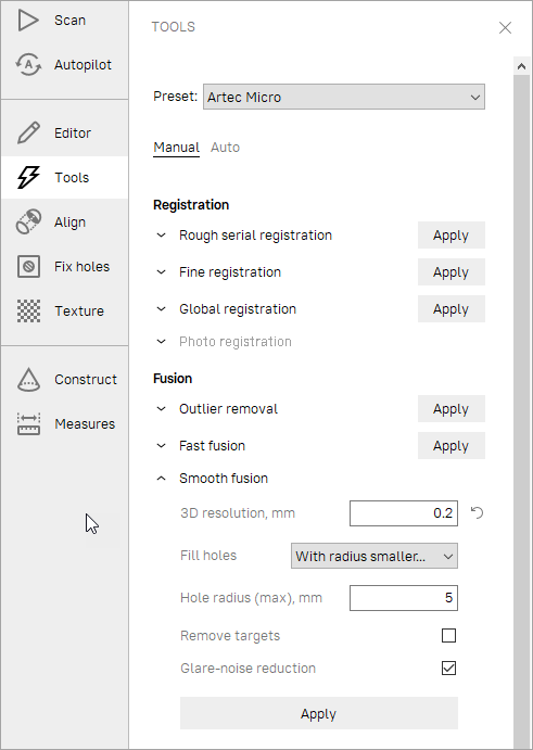
Figure 98 Tools panel: parameters of the fusion algorithm.

Fusion-Algorithm Errors

Occasionally, defects appear in the 3D model after fusion; some are correctable by creating additional scans, whereas others are correctable by using the model-processing tools described in the next section.

Figure 99 Surface noise caused by insufficient data (left) and improved model after adding one more scan (right).

Errors that can be corrected by capturing additional scans include low-amplitude noise on the surface (see Figure 99, left). Normally, this error indicates that the affected area has a small number of frames. The number of frames needed to eliminate the noise depends on the reflective properties of the object’s surface. To correct the error, you need one more scan to cover the noisy area (see Figure 99, right).

Sometimes the cause of noise is an insufficient number of scanning angles. Areas captured at a larger angle have more noise than areas captured at a direct angle (i.e., 90 degrees). You can correct this error by scanning the area again using a better angle.

When the scanning conditions or the object features are such that you are unable to capture additional data, you can correct errors using the Fix holes (see Hole Filling) or Smoothing (Smoothing (Tools)) tools. If such errors are frequent, reduce the speed at which you move the scanner around the object, or increase the capture rate (see Decreasing Scanning Speed).

Editing Models

The resulting fusion model may contain surface defects due to scanning or registration errors. Artec Studio provides a number of tools to correct such errors:

• Repair corrects the model’s triangulation errors.

• Small-object filter removes small objects located near the model surface.

• Fix holes semiautomatically fills holes and smooths the model edges.

• Hole filling fills holes in the model automatically

• Smoothing filters low-amplitude noise over the whole model

• Smoothing brush enables manual smoothing of the surface areas with the most noise

• Mesh simplification reduces the number of polygons in a model while minimizing lost accuracy

• Isotropic remesh creates isotropic mesh while keeping the processed mesh as close to the original as possible

Each algorithm processes all scans selected in the Workspace panel and replaces the original data with the results. If the algorithm is unsuccessful, you can restore the original data by clicking (Undo) in the Workspace panel.

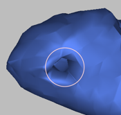
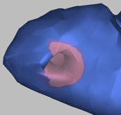
Small-Object Filter

If you forgot to erase outliers before fusion (see Eliminating 3D Noise (Outlier Removal)), Artec Studio may solidify and preserve them in the scene as small, distant fragments.

You can effectively remove these remaining outliers by using a filtering algorithm.

To remove these artifacts, select in the Workspace panel only the model you are currently editing, then open the Tools panel. Click Apply next to Small-object filter to run the algorithm (see Figure 100). A window containing algorithm settings will appear when you click . You can adjust the following parameters:

• Remove surfaces

  • The All except largest option from the dropdown menu instructs the algorithm to erase all objects except the one with the most polygons

  • Smaller than specified erases from the scene all objects whose number of polygons is less than the amount specified in the Polygon count (max) parameter.

• Polygon count (max) is the maximum number of polygons for Smaller than specified.

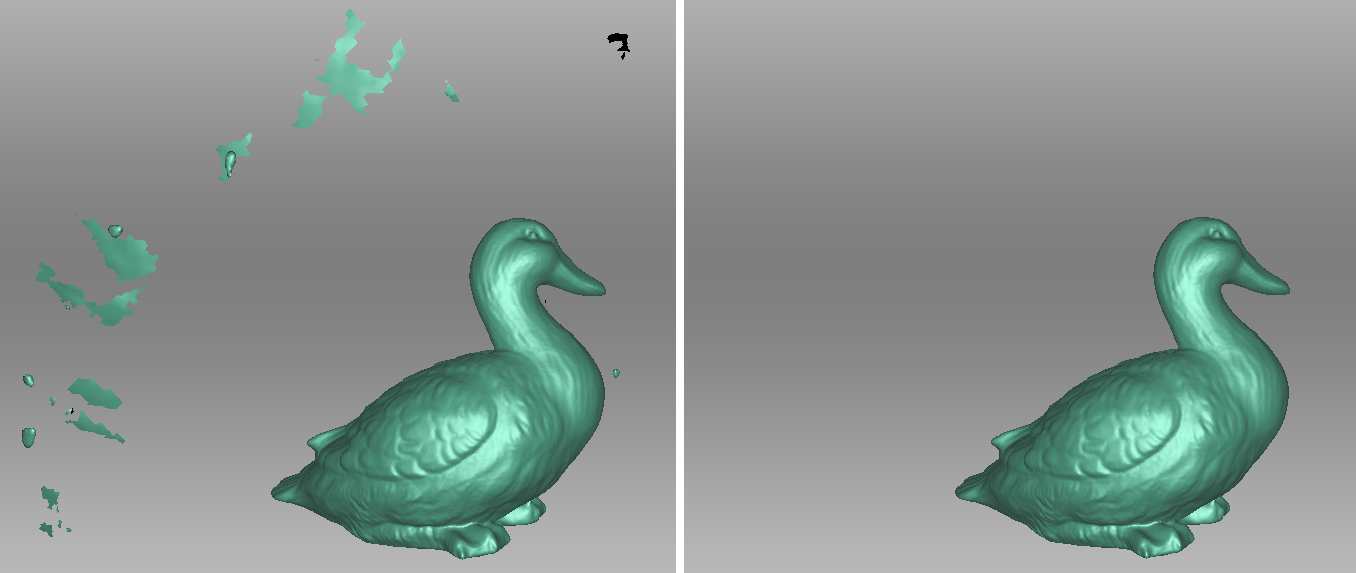
Figure 100 Filtering of small objects: before (left) and after (right).

Defeature Brush (Editor)

Erasing certain geometrical imperfections often demands further processing of the resulting holes in the model. The Defeature brush combines functions of the Eraser and Hole filling tools and may boost your productivity. To use it, follow these steps:

Warning

If you edit a textured model, note the following. Since the texture will incorrectly fit the altered surface, the Defeature brush will remove it from the model. So you will need to repeat texturing after you finish editing.

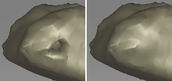
Figure 101 Defeature brush: imperfection on the scanned surface (left), results of applying the tool (right).

1. Select one model in the Workspace panel.

2. Open the Editor panel using the side toolbar and click either Defeature brush or hit D.

3. In the Editor panel, choose the required selection type.

4. Consult the instructions for each mode and select regions on the model that you want to modify. To clear all selections, click Deselect.

5. Click Apply. The software will delete the feature, close up the hole and smooth the surface.

To undo changes, click in the Workspace panel or menu Edit, or hit Ctrl + Z. Each click of the Apply button generates a command history entry. To undo several operations, use the dropdown menu of button and select the lowest entry.

Selection Types

Type	Illustration	Usage
2D		Hold down Ctrl and use Scroll wheel to adjust the tool size. Paint with Ctrl+LMB to create a selection.
3D		See above.
Rectangular		Use Ctrl+LMB to select a rectangular region.
Lasso		Use Ctrl+LMB to freely outline an irregular region. You can release LMB (not Ctrl) and then continue clicking on desired points to select a desired shape.
Cutoff-plane		Create selection as in 2D mode. Once you have released the mouse button, a plane will appear. If necessary, adjust the plane level by using Scroll wheel while holding down Ctrl+Shift or orient the plane freely in 3D space. To this end, hit Alt to display the designated control. Then still holding the key, drag the required control ring.

If you need to deselect any region, hold Ctrl + Alt and reselect this region. To clear all selections, click Deselect.

If the Select through checkbox is selected, all surfaces throughout the model are affected. If not, the brush only works on the visible surface.

See also

Hot keys in Editor.

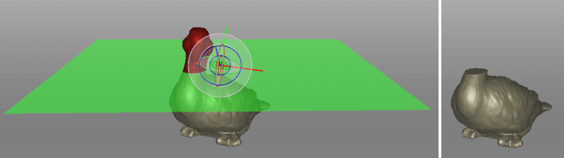
Figure 102 Applying Cutoff-plane selection in Defeature brush.

Smoothing

Smoothing (Tools)

The smoothing algorithm evens out noisy areas in the 3D model. Artec Studio provides two such tools: automatic smoothing of the entire model and manual smoothing of specific areas identified using a brush (see Smoothing Brush (Editor)).

To run the automatic smoothing algorithm, open the Tools panel and select Smoothing. You need only set the Steps parameter (the number of algorithm iterations to be performed).

Smoothing Brush (Editor)

The Smoothing brush is a tool that you can employ selectively in specific areas without touching areas that require no alteration (for more information about automatic smoothing, consult Smoothing (Tools)).

To use the Smoothing brush,

1. Select just one model.

2. Open the Editor panel, and click the icon or hit S.

3. Hit Ctrl, an orange region will appear around the cursor in the 3D View window.

4. Change brush size if necessary:

   • Use either the Ctrl + [ and Ctrl + ] shortcuts or

   • Use Scroll wheel.

   • Enter a size (in millimeters) in the Brush size field.

   • Alternatively, you can adjust the slider bar in the Smoothing brush panel.

5. Set the smoothing strength if necessary:

   • Enter the desired value in the Smoothing strength field or

   • Adjust the slider bar.

6. Hold LMB and paint the surface region in order to smooth it. The tool will smooth the affected areas (see Figure 103, right).

To undo changes, click in the Workspace panel or hit Ctrl + Z as many times as needed to return to the original state of the model since each brush stroke generates a command history entry.

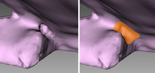
Figure 103 Before smoothing (left) and smoothing out a poorly captured area (right).

Smoothing Edges

The Edges tab allows you to smooth ragged edges of the model.

To smooth an edge or any part of it, follow the steps:

1. Open Fix holes → Edges. It will show the list of edges detected on the surface. These defects are sorted by their full length.

   • Mark the checkbox next to the edge in the list to select a whole edge 2.

   • In 3D View window, hold down LMB and drag the square control to specify a part of the edge.

   • Use the Select all button to select all edges.

2. Artec Studio will highlight these edges in red and draw yellow curves alongside them depicting smoothed boundaries.

3. Use the Strength slider to control the edge-smoothing intensity as necessary.

4. Click Smooth edges.

5. Click Apply to confirm the results. If the results aren’t satisfactory, use the button to cancel recent changes.

2

If the Move camera to selection option is checked, the model will automatically rotate to display the selected hole.

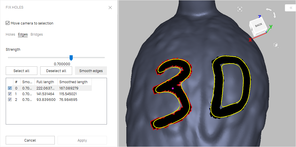
Figure 104 Boundary selection for edge smoothing

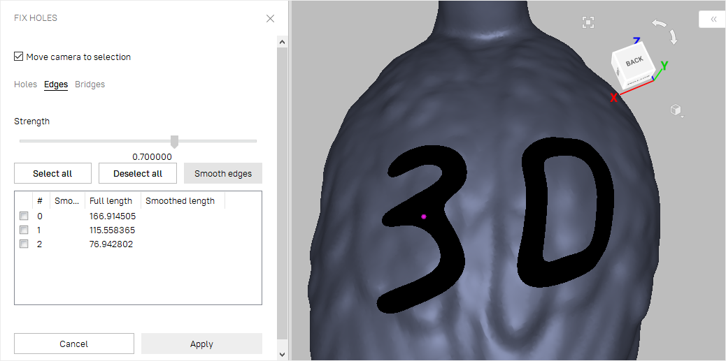
Figure 105 Edge-smoothing algorithm results.

Hole Filling

Sometimes the shape of an object or the scanning conditions prevent you from properly capturing of all parts of the scene. As a result, the fused 3D model will have holes. In such instances, you can use either of the hole-filling tools to interpolate the surface.

Bridges or Smart Hole Filling

The Bridges tab is intended to connect a pair of the edge fragments by constructing a surface that follows the curvature of the neighboring surfaces.

To create a bridge, follow the procedure:

1. Open Fix holes → Bridges. All holes will outline in red.

2. Specify two opposite fragments 3 between which a bridge will go (Figure 107). There are two ways to do this:

   Quick method	Ctrl-key method
   Perform the steps below for each fragment:	Click once anywhere in the 3D View to activate this method and then perform the steps below for each fragment:
   Point the cursor at the edge. A part of this edge will be automatically highlighted indicating a future fragment. Drag the cursor along the edge to find the desired fragment location. Click LMB to confirm the fragment.	Press and hold Ctrl and then point the cursor at the edge. Press and hold Ctrl+LMB to specify a fragment beginning. Still holding Ctrl+LMB, drag the cursor to specify the entire fragment. Release Ctrl+LMB to confirm the fragment.

3. Once you’ve confirmed the second fragment, a bridge preview will appear.

4. Drag the square sizing handles to adjust the bridge width and position as necessary.

5. Adjust bridge curvature on both sides and Bridge smoothness as necessary.

6. Click Build bridge to confirm your bridge.

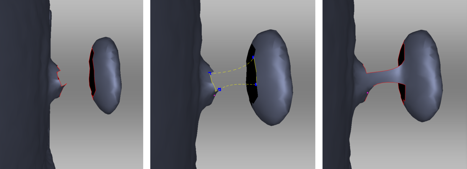
Figure 106 From left to right: original surfaces, bridge preview, actual bridge.

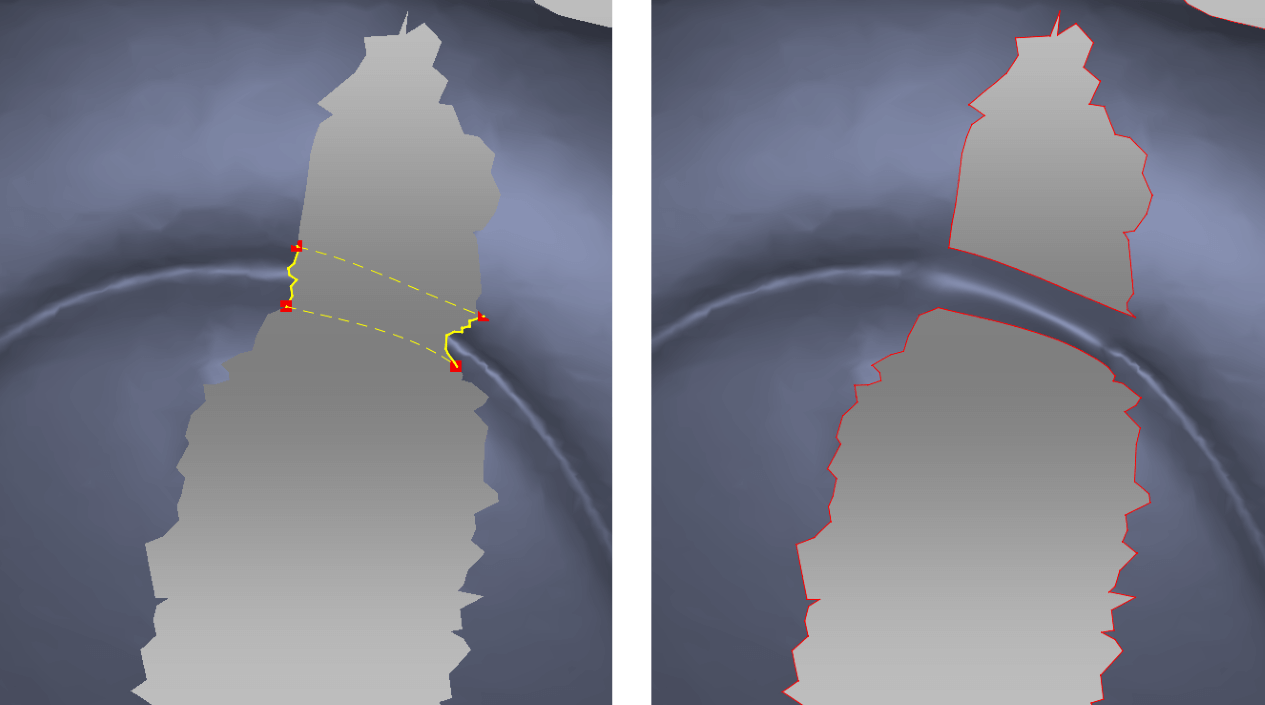
Figure 107 Specifying fragments. Correct fragments can resolve original geometry.

The table below lists the possible actions matched with the options and commands for this tool.

Prepare edges by removing raggedness	Select the Smooth edges first checkbox
Preserve the original geometry (Figure 107)	Clear the Smooth edges first checkbox
Smooth bridge surface	Use the Bridge smoothness slider
Edit bridge-preview position	Drag the square controls around the corners of the bridge preview
Adjust bridge tension	Use interactive sliders Curvature (start, end)
Delete bridge preview	Click Clear preview or Delete key

3

Normally a bridge goes between two opposite fragments of one hole. In complex cases, you may use fragments on different holes or edges.

Smoothing or Keeping Edges

Smoothing edges might not always be beneficial to you. If the bridge failed to recreate the original geometry, try one or several actions from the following list:

• Clear the Smooth edges first checkbox.

• Use small or medium values of the Bridge smoothness slider (Figure 108).

• Select fragments correctly.

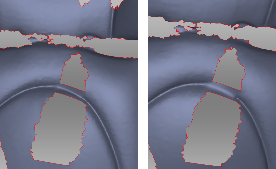
Figure 108 Small smoothness values on left and maximum on right.

Automatic Hole Filling

To quickly and automatically fill holes, use the Hole filling algorithm in the Tools panel. The algorithm only processes holes with perimeters below the threshold specified in Hole perimeter (max), mm (maximum length of the hole perimeter in millimeters).

Use button to access this parameter.

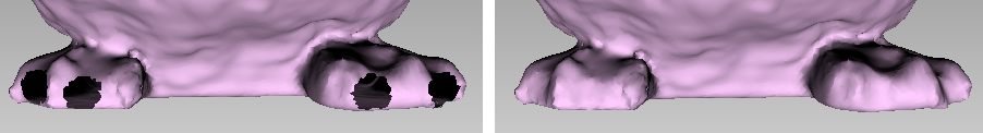
Figure 109 Hole-filling algorithm: original model on left, processed on right.

Fixing Holes

Unlike Bridges, the Holes tab provides flat hole filling.

1. Open Fix holes from the side panel.

2. Select the Holes tab. It will show the list of holes detected on the surface. These defects are sorted by their perimeter length.

3. Select a hole either in 3D View window or mark the checkbox next to it in the list. Artec Studio will highlight these holes in red (see Figure 110).

   Note

   If the Move camera to selection option is checked, the model will automatically rotate to display the selected hole.

   Hint

   Use the Select all and Deselect all buttons in the panel to select or clear all selections, respectively.

4. Click Fill holes to repair your model.

5. Click Apply to confirm the results. If the results aren’t satisfactory, use the button to cancel recent changes.

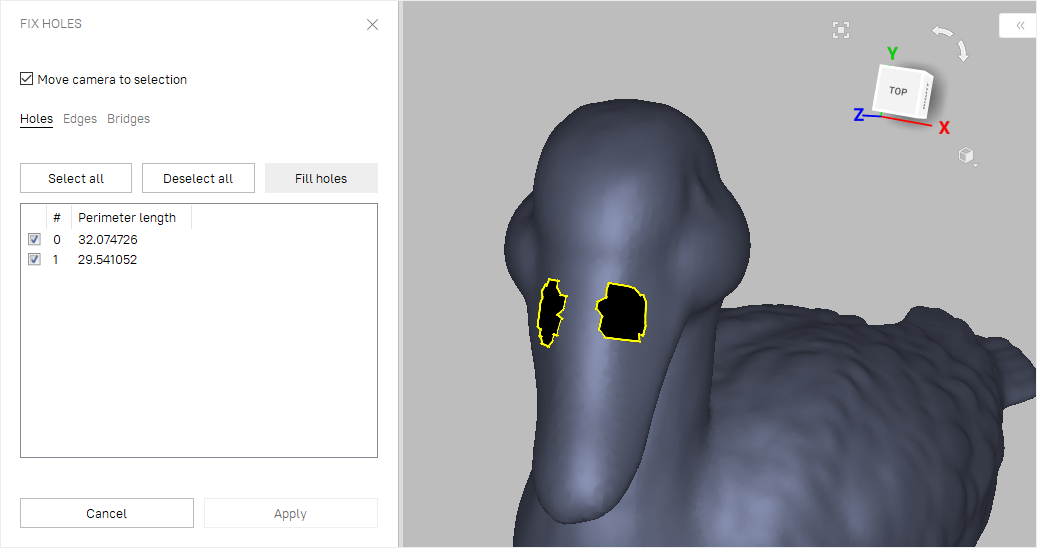
Figure 110 Two holes marked for correction.

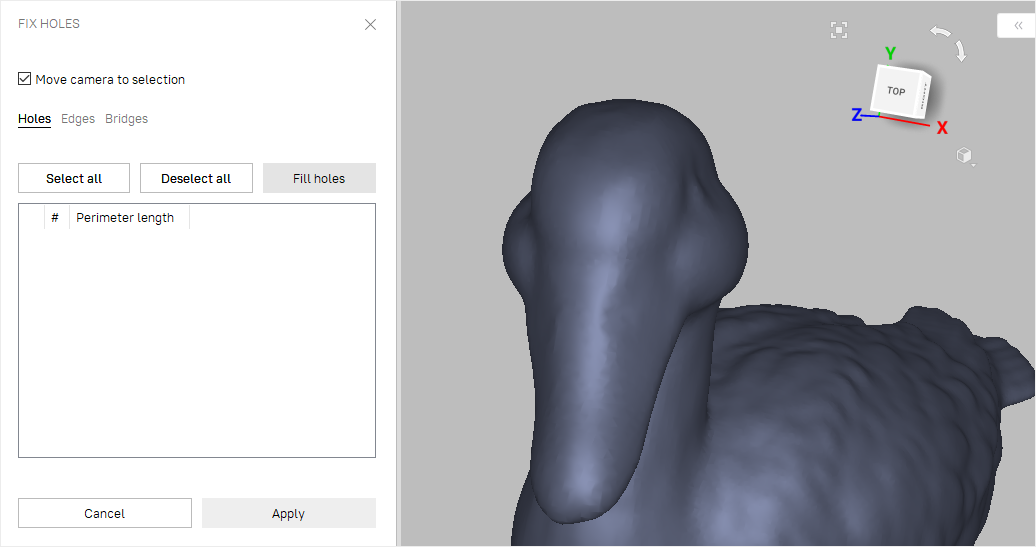
Figure 111 Result from running the Fill holes algorithm.

If you try to exit the Fix holes mode without accepting changes, the software will ask you for confirmation.

Mesh Simplification

The mesh produced after fusion may be less than optimal for some applications because it will contain a large number of polygons. This complexity will increase the amount of memory the model occupies, hindering further processing. To optimize the model size while retaining accuracy, use the Mesh simplification algorithm.

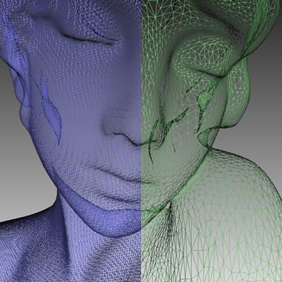
Figure 112 Mesh simplification: original mesh on the left, optimized mesh on the right.

Select the model and open the Tools panel. You can choose from two algorithms.

Conventional Algorithm

Open the dropdown algorithm settings by clicking the button next to Mesh simplification. Select the appropriate processing method (determined by the Target when simplifying):

• Shape deviation optimizes model to a predetermined accuracy: the Maximum shape deviation, mm parameter defines the optimized model’s maximum allowable deviation (in millimeters) from the original model. When the algorithm reaches this value, the optimization stops.

• Remove small polygons performs simple mesh optimization, removing triangles whose edge lengths are less than the Polygon edge length (max), mm value (in millimeters).

• Polygon count simplifies the model by targeting the number of triangles specified in the Polygon count text box. The algorithm minimizes the resulting model’s deviation from the original model, but the final deviation value will remain unknown until processing concludes. Use this method when you know how many triangles the resulting model should have.

  Tip

  To determine the number of triangles, reveal the Properties panel for the appropriate model in the Workspace panel.

• Keep texture is similar to the Polygon count algorithm, but intended for meshes with textures mapped by the Atlas method (see Applying Texture (Procedure)). This approach not only simplifies the polygon grid, reducing the number of triangles, but it preserves texture.

Tip

Since the UV methods tend to slightly reduce texture resolution, we recommend using either of them only when no raw scans are available. It is generally better to simplify models using one of the regular method and then reapply texture.

The three first algorithms in the list above have the additional parameter:

Keep edges maintains the model boundary. Mesh simplification on the scan edges may affect their geometry. Thus, if the shape of the boundaries is more important than the optimized mesh, select this checkbox. Otherwise, clear it, and the algorithm will simplify the boundary mesh.

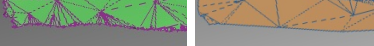
Figure 113 Boundary-appearance options: Keep edges enabled (left) and disabled (right).

After adjusting the algorithm settings, click Apply to start processing.

Note

Mesh simplification may take a long time when the parameters of the original and optimized models are significantly different (for example, if the deviation value is high in Shape deviation mode or if the required number of polygons in Polygon count mode is much smaller than the number in the original model). For very large 3D models the operation requires extensive memory resources and may fail owing to insufficient RAM. Free the memory by closing unused applications and by optimizing memory usage in Artec Studio, keeping in mind the recommendations in Memory Management: Smart RAM Usage and History of Project Changes.

Fast Mesh Simplification

The Fast mesh simplification algorithm works faster than the conventional one. To run it, perform these steps:

1. Open the dropdown algorithm settings by clicking the button next to Fast mesh simplification.

2. Specify in the Polygon count text box the desired number of triangles for the resulting model. You can determine how many are in the actual model by double-clicking it in the Workspace window.

3. Set the Nonstrict polygon count option:

   • If this checkbox is cleared, the value specified in the Polygon count text box remains constant.

   • If this checkbox is selected and the algorithm is unable to produce a surface with the specified number of triangles (Polygon count), Artec Studio will automatically update this value. In other words, improving the quality of the resulting surface is the primary objective.

4. Click Apply to run the algorithm.

Photo Registration

The photo registration algorithm Artec Studio enables you to apply textures to models using photographs. Photos of the object can be used to project textures onto fused models. This advanced texturing approach can be used to capture complex textures and significantly enhance models.

Preparing Object

To obtain best texturing results, it is important to follow the below given tips before scanning and taking photographs.

1. Before taking photos, make sure the object has prominent texture features.

2. For large objects with monochromatic surfaces, add additional features in the background to highlight the texture. However, if you will have to rotate the object, it is better to use a plain background.

3. Provide adequate and uniform lighting. It is recommended to use external studio lighting for cameras with low light-sensitivity. Do not use the flash.

4. In the case when exposure is too big to hold the camera in hands, it will help to use a tripod.

5. Make sure the object remains stationary during scanning and taking photos. If you need to turn or move the object to scan all sides, it is recommended to take photos immediately after scanning in one position, before moving the object to scan in another position.

Capturing Photos

The photos for registration can be captured using any SLR camera or a smartphone with a good camera. For optimal results, it is important to capture good quality photos that are sharp and bright, and not noisy and blurred. Here are some best practices for capturing good quality photos for texturing.

1. Capture photos from a proper and fixed distance. The object must be at the center of the photo and occupy the most space, with minimal background details.

2. Adjust and fix the focal length, exposure and aperture.

   Note

   All photos must be of the same focal length and resolution for proper registration.

3. Do not rotate the camera or change the orientation. Capture all photos either vertically or horizontally.

4. Capture subsequent photos of the object with at least 66% or 2/3 overlap while moving the camera. Take a series of photos, much like the texture frames captured by Artec scanners.

5. Photograph each element of the object at least 3 times.

6. Avoid taking photos of any additional objects that can disturb the texture of the object you’re scanning, like a pedestal the object is placed on.

7. It is recommended to convert all photos to .jpeg format and preserve their EXIF information.

Color corrections or white-balance corrections can be applied to photos for post-processing, but it is advisable to process all the photos in the same manner. Avoid geometrical transformations, resizing, distortion corrections, or color-space transformations.

Applying Texture (Procedure)

After all the necessary photos have been captured, save them in a folder in your system. Obtain the 3D model of the object using the standard procedures until fusion, and then to apply photo texture, do the following:

1. Go to File → Import, and click on Import photos. Select all the necessary photos, and they will appear in the workspace.

   Note

   The photo registration algorithm does not accept photos from different cameras at a time. At a time, import or select photos captured with one camera only.

2. In the worksapce, select all the scans of the model, the fusion and the photos (all three items).

3. Open the Tools panel, and locate the Photo registartion section.

4. Set the photo registration parameters as necessary. See Photo-Registration Parameters.

5. Click Apply.

6. Once the photos are registered, follow the Texturing procedure, and apply the texture to the model.

Photo-Registration Parameters

Preprocess images	On/Off	Enable it to apply contrast to scanner images. For Eva, Leo, or Spider (if the object was captured from large distances and the textures are dark).
Describer preset	Normal, Medium, or High	You can choose presets to enhance the textural information for registration. Higher preset corresponds to higher number of features and lower threshold. In other words, for photos with high number of features, select ‘High’ and so on.
Camera field of view		Artec Studio determines this value automatically using photo metadata. However, in case of erroneous metadata, enter the accurate field of view of the camera (in degrees).

Texturing

Artec scanners are equipped with a color camera, allowing you to capture 3D surfaces with texture and expanding the range of objects available for scanning. Texturing is a process that projects textures from the individual frames onto the fused mesh.

Preparing Model

To take advantage of texture, do the following:

1. Make sure the Don’t record texture checkbox is cleared.

2. Adjust the capture frequency for texture frames if necessary (see Texture-Recording Mode or Frequency for Capturing Texture Frames).

3. Avoid turning off the flash bulb.

4. Adjust the texture brightness in Preview mode by using the eponymous slider in the Scan panel.

5. Scan the object using a tracking algorithm of your choice. Captured frames are marked with the checkerboard icon in the Workspace panel (surface-view mode) (see Figure 57, right).

6. Process the data and create a model, consulting the list in the beginning of Data Processing or Use Autopilot.

7. Run a mesh-simplification algorithm for the resulting model (see Mesh Simplification) to accelerate the texturing process.

8. Use the Texture panel to apply the texture to the model.

Applying Texture (Procedure)

The 3D model obtained after fusion contains no texture information. To apply textures onto a model, do the following:

1. Open the Texture panel.

2. Choose a model from the first list (see Figure 114); Artec Studio will apply the textures to this model.

3. From the second list, select the scans from which you created the model (these scans have the required textures 4) or the photos you registered using photo registration.

4. Next, choose a method for applying textures to the model. Artec Studio offers two methods:

   • Preview (triangle map)

   • Export (texture atlas)

5. Select the required Output texture size 5 and other options as necessary (Supplementary Settings).

6. Click Apply to start the texturing process 6.

7. Finally, when the texture is ready, adjust it as necessary.

4

Note that those texture frames from Leo scans that appear blackish when previewing them in the 3D View window will not be used for texturing the model (see Specifics of displaying the textures of Leo scans for details).

5

Texturing with the 16K resolution (16384x16384) is only available if your graphics card features at least 3 GB of GPU memory.

6

To optimize resource utilization, Artec Studio unloads all surfaces from memory, except those needed for texturing, before running the applying procedure. For a more detailed description of selective project-data loading, see Memory Management: Smart RAM Usage.

To reduce or increase the resolution (Output texture size) of the already applied texture, you can re-apply it several times faster by enabling the Export (reuse UV map) option.

To replicate texture from a textured model instead of raw scans, use the Export (transfer from model). Ensure that you’ve selected this model in the Select texture source field. Using texture from a textured model might be useful in the following cases:

• Original scans are lost.

• Intention to replicate texture altered using Texture healing brush.

• Speed up texturing identical models or models undergone Defeature brush operations.

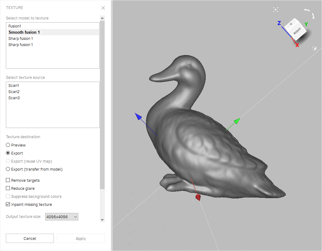
Figure 114 Choosing a texture-application method and adjusting its parameters.

Warning

We recommend that you avoid applying texture to models that have undergone major changes in geometry or orientation. The algorithm will apply the texture incorrectly if you have done any of the following:

• Position or transform the model relative to its source scans

• Nonrigid Alignment

• Erase major parts of the model

Perform these operations only after texturing.

Modes

Table 14 Comparison of the texture-applying methods.

Mode	Texture Distortion	Speed	Number of Textures	Texture-Resolution Management
For preview	Does not preserve aspect ratio of triangles	Fast	One or more	Adjust triangle size and texture-image resolution
For export	Preserves aspect ratio of triangles	Slow	Only one	Adjust texture-image resolution

Texturing for Preview (Triangle Map)

The Preview method transfers all textured triangles to a square texture image (or a series of images). You can adjust the Triangle size (in pixels) 7 using the eponymous slider (see Figure 115, right). To select the resulting texture size, use the dropdown list (maximum texture size depends on the capabilities of your graphics card). After changing the triangle/texture size, the estimated number of textures will appear in the Estimated area at the bottom of the panel; the actual number may differ slightly, however.

7

Triangle size is determined by the number of pixels per side.

Texturing for Export (Texture Atlas)

The Export method cuts the surface into pieces, then unfolds and nests these pieces flat and fits them into the specified image size (see Figure 115 (middle) and Figure 69 in Displaying Boundaries of Texture Atlas). This method takes longer to run than Preview, but the resulting texture is much more convenient for manual editing.

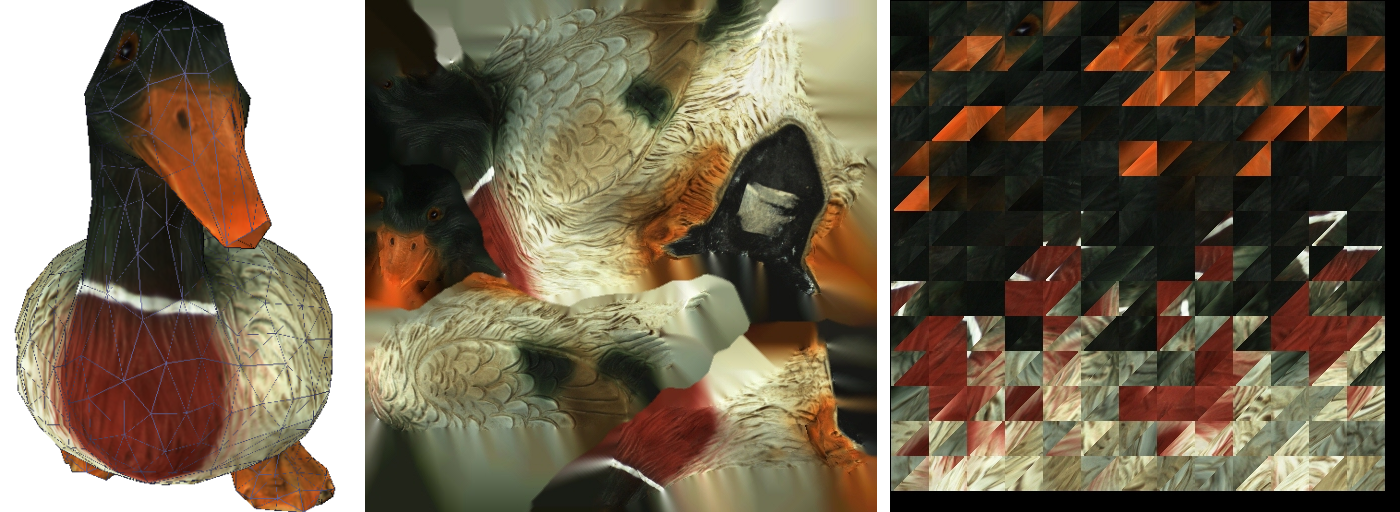
Figure 115 Texture mapping methods: mesh with texture applied (left), texture-atlas sample (middle) and triangle-map sample (right). The latter covers only a portion of the mesh surface (the rest two images not shown).

Supplementary Settings

To modify a texture using an inpainting technique, use one of these two options:

Inpaint Missing Texture

This option allows you to apply a texture to regions with no texture information by spreading it from the neighboring regions.

Remove Targets

Remove targets is similar to inpainting. It paints out targets by applying surrounding texture information (targets are used to facilitate scanning—see Target-Assisted Scanning). This option makes sense if you enabled Remove targets before producing this fusion model (see Creating Models (Fusion)).

Enable Texture Normalization

Enable texture normalization aims to compensate for uneven lighting caused by movement of a scanner’s flash unit during capture. We don’t recommend clearing this checkbox.

Reduce Glare

Reduce glare is intended to eliminate glare spots on texture. This option is only available for Texturing for Export (Texture Atlas) and requires many texture frames captured from different perspectives.

1. Check whether the source scans include sufficient number of frames (especially texture frames). If necessary, increase texture-frame rate and rescan.

2. Select the Reduce glare checkbox.

3. Adjust the Reduction level slider as necessary. Avoid extreme values.

Hint

Glare reduction is a time consuming algorithm. If you plan to obtain a high-resolution texture, we advise you to first tweak the settings on low values (for example, 512 x 512) and then reapply texture with the required Output texture size.

Suppress Background Colors

Object’s surfaces may inherit texture information from the surroundings. To diminish this impact, use the Suppress background colors option. This option is only available for Texturing for Export (Texture Atlas), requires the enabled Reduce glare option and a sufficient number of texture frames captured from different perspectives.

1. Ensure the Reduce glare checkbox is selected.

2. Select the Suppress background colors checkbox.

3. Adjust the Reduction level slider as necessary. Avoid extreme values.

Figure 116 Diminishing background color impact.

Texture Adjustment

After the texturing is complete, you can adjust the texture on the model (see Figure 118).

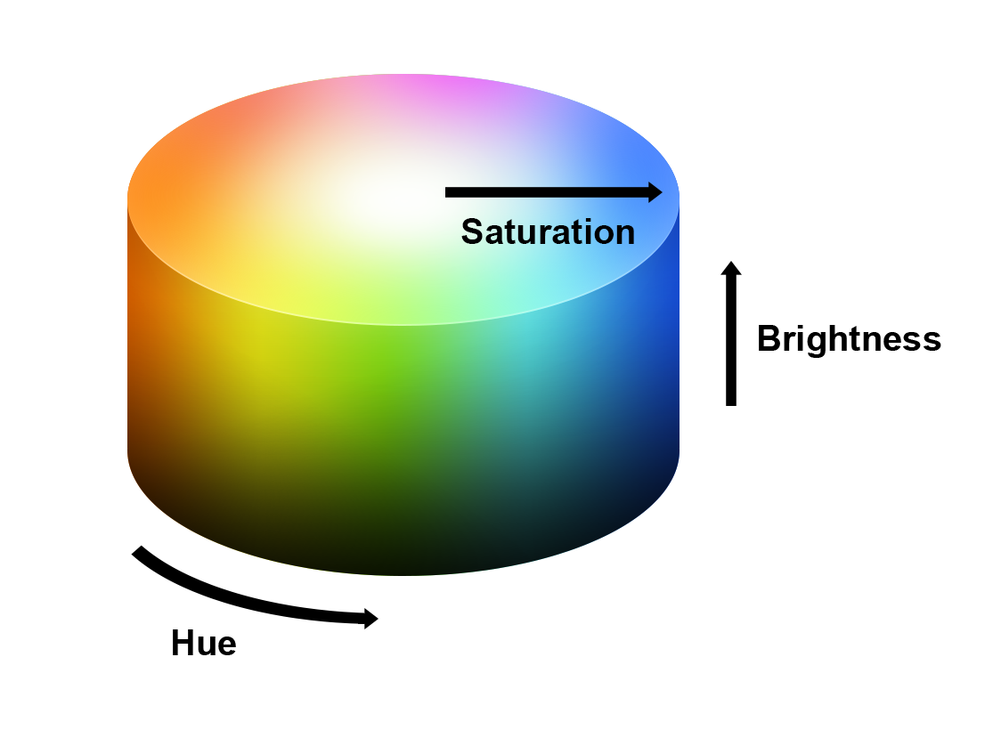
Figure 117 Hue, saturation and brightness representation.

You can adjust the following texture parameters by way of the corresponding sliders (see Figure 117 for details):

• Brightness

• Saturation

• Hue

• Contrast

• Gamma correction

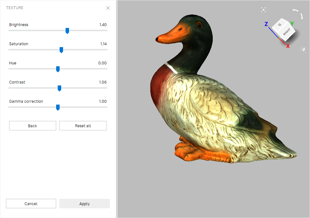
Figure 118 Texture adjustments.

The initial position of the Hue slider corresponds to the current texture color. Dragging it left or right corresponds to rotation counterclockwise or clockwise, respectively, on the color wheel.

After making the necessary changes, click Apply to transfer the resulting textured model to the Workspace panel.

To reopen the texture-adjustment dialog, follow the steps:

1. Select a textured model in Workspace.

2. Use RMB to call the context menu.

3. Select the Adjust texture command from the list.

Texture-Healing Brush: Manual Inpainting

You can manually inpaint missing textures by using the Texture-healing brush. This tool is based on the same algorithm as the Inpaint missing texture option covered in Applying Texture (Procedure). The inpainting algorithm uses texture information from neighboring regions to fill in areas with missing or incorrect texture. Left image in Figure 119 shows a small texture imperfection: a felt-tip pen mark on the figurine. Results of inpainting this region appear in Figure 119 (right).

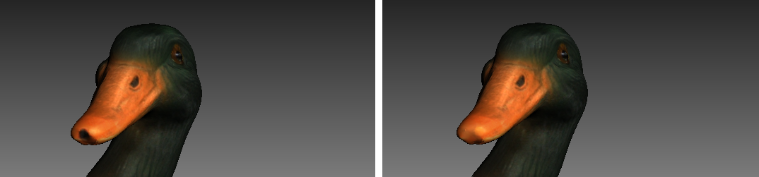
Figure 119 Texture-healing brush: before application (left) and after (right).

To launch the tool and inpaint a texture, do the following:

Hint

We advise you to first back up your model by selecting the Duplicate scans command from its context menu since the undo function is unavailable in this tool.

1. Mark the model textured for Export with the flag.

   Important

   This version of Artec Studio does not support texture restoration on the models ‘textured for Preview’ (triangle map) and in regions of any models that have been corrected using the Defeature brush.

2. Open the Editor panel by clicking its icon in the side toolbar.

3. Select the Texture-healing brush.

4. Hold down Ctrl while using Scroll wheel or [ and ] keys to adjust the tool size. It should not exceed the size of the region that needs texture correction.

5. Paint over the region of interest using LMB while holding down Ctrl so that the tool (a circle or a spot) only rolls over the problem area. Try to avoid touching neighboring areas. Use the Deselect button to clear all the selections.

6. Repeat the previous step as necessary.

7. Click Apply to accept the changes or close the panel to reject them.

Note

If you paint an area in which the number of polygons exceeds the value specified in the settings dialog (see Warnings), a message will appear prompting you to either ignore the value, which means that processing may take longer, or cancel the operation.

Preparing Models To Export

Moving, Rotating and Scaling (Transformation Tool)

The Transformation tool allows you to move, rotate, scale and mirror objects relative to the global coordinate-system axes.

To access this tool, open the Editor panel and select Transformation tool or hit T. The panel will open, displaying four tabs that correspond to different modes for altering the object position in the global coordinate system. The name of the active mode appears at the bottom of the 3D View window.

To revert your changes inside the tool, use the Reset button. Artec Studio applies changes when you leave the tool. Use the (Undo) button in the Workspace panel or hit Ctrl+Z to reset changes after you close the tool.

Hint

To quickly move objects to the origin and align them with the camera viewport, use the Auto-position button.

Note

The Transformation tool does not affect objects with the Locked position status (). See Locking Object’s Reposition for details.

Translate

To enter translation mode, click the Translate tab or hit T. Three input fields will appear in the Editor panel showing the current origin coordinates (in millimeters) of the local coordinate system. The initial position of the local coordinate system will be in the center of the global one. To translate an object, do either of the following:

• Enter the new coordinate values for the local system using the input fields in the Editor panel. To adjust the position only along a specific axis, first hit the corresponding X, Y or Z key.

• Translate the object in the 3D View window by dragging the corresponding control (see Figure 120):

  • Square in the center to move it freely

  • Arrow to move it along a specific axis

  • Lines between arrows to move it along the two axes simultaneously

Note

Orienting the object may be easier if you first specify a new position for the origin of the local coordinate system: double-click on the desired surface point in the 3D View window.

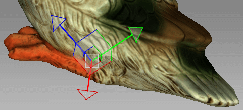
Figure 120 Translation control

Rotate

To enter rotation mode, click the Rotate tab or hit R. Three input fields containing the Euler-angle values will appear in the Editor panel. Initially, all values are set to zero. To rotate the object, do either of the following:

• Enter the new angle values (in degrees) using the input fields in the Editor panel.

• Drag one of the three circles (see Figure 121) to rotate the object. Hitting the key that corresponds the required axis (X, Y or Z) will hide the controls for the other axes.

Note

Orienting the object may be easier if you first specify a new position for the center of the local coordinate system: double-click on the desired surface point in the 3D View window.

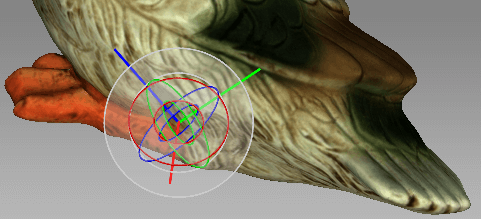
Figure 121 Rotation control

Scale

To enter scaling mode, click the Scale tab or hit S. A single input field with the current scale value (1.000) will appear in the Editor panel. You have two options for scaling the object:

• Enter the new scale value in the field.

• Drag the origin of the control (Figure 122) or either of its round ends in the 3D View window.

Figure 122 Scaling control

Placing Objects on Coordinate Plane (Positioning Tool)

You may need to place the model on one of the coordinate planes (e.g., for aesthetic reasons or when preparing the model for measurements, for capturing a screenshot, for exporting and so on). Instead of adjusting the model position using the Rotate and Translate modes of the Transformation tool, you can use the special Positioning tool. To do so, follow these steps below.

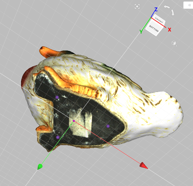
Figure 123 Positioning the model in the global coordinate system.

1. Open the Editor panel from the side toolbar and click either Rough positioning button or hit P.

2. Choose the Rough tab—a rough positioning is available for all the object types, whereas the Precise option works only with CAD objects.

   See also

   Setting constraints for CAD primitives

3. Ensure that the coordinate axis grid is shown. Otherwise hit G or select the Grid command from 3D toolbar.

4. Choose the coordinate plane in which you want to place the model by activating one of the following options: XOY, YOZ or ZOX. Note that you may skip this step and return to it after Step 3.

5. Use LMB to specify at least three points on the surface; the plane will automatically pass through their center of mass (see Figure 123). The following conditions will then apply:

   1. For each additional point you specify, Artec Studio rebuilds the plane. Click Clear points at any time to redefine the points.

      Note

      Three points determine a plane. When you’re dealing with nonplanar surfaces, however, three points may be insufficient. In that case, the more points you specify, the more precisely a plane will fit the surface.

   2. In addition to the plane passing through the center of mass of the points you select, the coordinate origin will shift to that location as well.

   3. The position of the coordinate origin is adjustable, as described below.

6. Invert the direction of the coordinate axis, if desired, by clicking the Invert Z button for the XOY plane, Invert X for YOZ, or Invert Y for ZOX.

7. If appropriate, adjust the model’s position relative to the coordinate origin:

   1. Shift + LMB—rotate the model around the axis that is currently normal to the plane

   2. Shift + RMB—move the model along the plane in a fixed direction

   3. Shift + LMB + RMB—move freely along the plane

8. Hit Apply to fix the model on a specified plane or close the panel to cancel positioning.

To discard changes of object position, hit Ctrl+Z.

Tip

The Enable automatic base removal option may come in useful to position scans automatically after the scanning completes (see Base Removal: Erasing a Supporting Surface.)

Note

The Positioning tool does not affect objects with the Locked position status (). See Locking Object’s Reposition for details.

Advanced Techniques

Automatic Processing

See also

Use Autopilot

Automatic processing is a special mode for the Tools panel that saves time and simplifies postprocessing. It allows you to run all postprocessing algorithms from the Tools panel (Rough, Fine and Global registration; Fast, Smooth and Sharp fusion; Small-object filter or Outlier removal; Hole filling; Mesh simplification and Smoothing) with a click of just one button.

Each algorithm setting and parameter is based on the values for a preset configured in the manual mode. To change these values:

1. Switch to Manual mode.

2. Select a specific scanner type via the Preset dropdown list.

3. Use the expand button to reveal parameters for the required algorithms.

4. Make the necessary alterations and click Apply.

5. Switch to Auto mode.

6. Select the checkboxes near the algorithms you intend to run.

7. Click Go! to begin automatic processing.

Changing the scanner preset type resets all the parameters to the default ones (for the selected preset).

Figure 124 Manual adjustment for the specific scanner type.

Keep in mind that the algorithms run in the order in which they are listed, starting with Rough serial registration and ending with Isotropic remesh. Thus, if you want to run the Small-object filter before Fast fusion or Global registration, for instance, you must do so manually.

Unlike manual processing, automatic processing runs without the need for constant user attention, so it is more convenient when processing large objects: you can configure the settings, start the process and leave it unattended. It can also process objects of any size, reducing the number of mouse clicks to get the result.

Mirroring

Artec Studio allows to mirror the 3D data. The application uses the local rotation center as a mirroring center (see Global Coordinate System and Rotation Center). If it isn’t specified, Artec Studio employs the global coordinate center.

To mirror the model, follow the steps:

1. Open Editor

2. Access Transformation tool

3. Select the Mirror tab

4. If necessary, double click the model to specify a rotation center

5. Select an axis to mirror the object along. Press the respective button—for example, Along axis Y.

Figure 125 Mirroring in action.

To revert your changes, use the Reset button. For details, consult Moving, Rotating and Scaling (Transformation Tool).

Isotropic Remesh

Isotropic remesh is an operation that modifies 3D model in the way that new mesh triangles have uniform size. Software packages where the models from Artec Studio are intended to be used may impose these requirements.

The algorithm produces an isotropic mesh, but doesn’t necessarily decrease the polygon count. However, the output file is often smaller than the original one through the uniform triangles.

Figure 126 Isotropic remesh operation in action: original model on left, processed one on right.

To produce a uniform mesh,

1. Mark the model using the flag

2. Open the Tools panel

3. Locate the Isotropic remesh section

4. Click and specify 3D resolution, mm as necessary

5. Click Apply.

Normal Inversion

Normal direction determines the visibility of a surface in 3D graphics. Learn how to show normals of the objects in Artec Studio 3D View, see Representation of Normals and Boundaries.

Normal inversion allows one to turn the model inside out. This operation may be useful when you need to manufacture some mating parts, like molds; or obtain a model based on its cast (e.g., turn the footprint cast into a shoe last, see Figure 127).

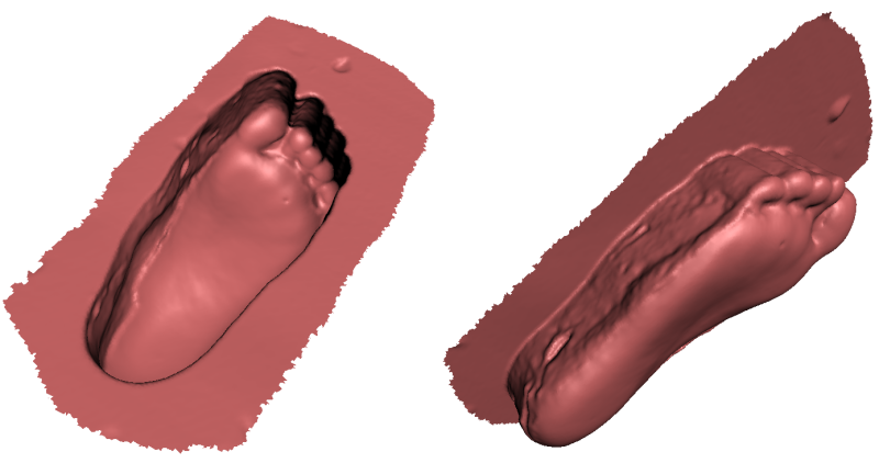
Figure 127 Normal inversion application: obtaining a foot model (right) from its cast (left).

To invert normals on a particular model,

1. Mark the model using the flag

2. Open the Tools panel

3. Locate the Normal inversion section

4. Click Apply.

Correcting Triangulation Errors

Some algorithms may introduce triangulation errors into the resulting model. These errors include the following:

• Unattached vertices. Points that are not vertices of any of the triangles

• Vertices with identical coordinates. Vertices that have the same coordinates

• Faces containing invalid vertices. Triangles that point to nonexistent vertices

• Singular faces. Triangles for which at least two of the three vertices coincide.

• Faces with equal signature. Faces with fully coinciding sets of vertices

• Edges incident to three or more faces. Edges that are adjacent to three or more faces

• Faces with wrong orientation. Faces whose normals point in a direction opposite to those of the adjoining faces

To correct these errors, mark a model in the Workspace panel by using the flag and hit Ctrl + R or select the Window ‣ Repair menu command. If the algorithm detects no triangulation errors, Artec Studio will notify you that it has found no defects. Otherwise, the Repair panel will open, displaying the above-mentioned list of defects to be corrected. Next to the names of the defects, a column will appear stating the number of defects of a certain type found in the model. You can select all defects by pressing View all. Doing so will display in the model all the defective vertices and triangles using colored points. You can disable display of any particular defect type by removing the icon next to the corresponding name, or disable them all by clicking View none. To correct the defects, click Repair all. Clicking the Apply button accepts the changes.