Data Processing
Once you have captured an object from all desired angles and created a sufficient number of scans, you can then build a 3D model. This chapter offers a detailed description of the process. Most of the examples herein use a decorative plastic duck figure as the test object (see Figure 72.).
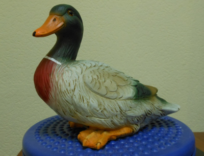
Figure 72. Target object: a decorative duck figure.
The process of creating the final model includes the following stages:
See also
- Revising and editing the data (Revising and Editing Scans)
- Scan alignment (Scan Alignment)
- Global data registration (Global Registration)
- Fusion of data into a 3D model (Fusion)
- Final editing of the 3D model (Editing Models)
- Texturing (Texturing)
Revising and Editing Scans
After each scanning session, Artec Studio saves the sequence of frames as a separate scan. The list of all scans for a given project appears in the Workspace panel (see Figure 73.).
Data in the Workspace panel is arranged in several columns:
- Selection flag
- —scans marked with a
 in this column will appear in the 3D View window and will undergo processing by all Artec Studio algorithms and tools.
 - Color
- —in this column, each scan has a colored square next to it. The square’s fill depends on the number of scan frames loaded into the application. When all frames are loaded, the square will be completely filled in. When only key frames are loaded, it will be half filled, and when all the scan data is unloaded, it will be unfilled (see Selectively Loading Project Data). You can change the scan color by clicking on the corresponding square and selecting the desired color from the palette.
- ID
- —ID number of the scan.
- Title
- —when a scan is created, Artec Studio automatically assigns it a name, such as Scan1, Scan2 and so on, according to the values in the Prefix and Start with fields in the Scan panel. To rename a scan, select it by left-clicking on its name. Then either hit
F2or right-click on the scan name to open the dropdown menu. Select the Rename... option. Both approaches open a dialog that allows you to specify the new name. - Loaded
- —number of scan frames loaded into memory (see Selectively Loading Project Data).
- Total
- —total number of frames and size of a particular scan (in MB).
- Max error
- —the largest registration-error value among all frames in the scan.
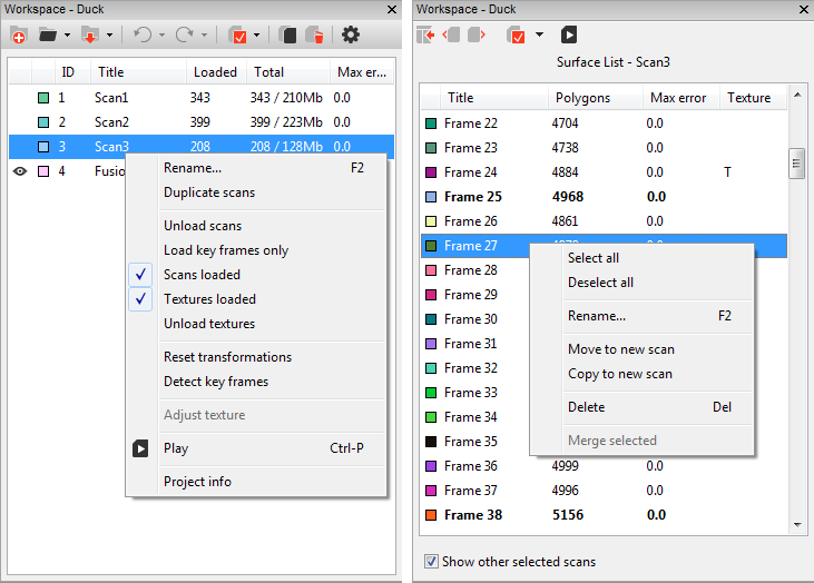
Figure 73. Workspace panel: scan list (original view) on left and surface list on right.
Selecting Data
Selecting Scans
Note
To view a scan in the 3D View window or to process it using a tool, first mark it with the icon.
| Purpose | Method | Alternate Method |
|---|---|---|
| Select scan in Workspace | Left-click on the scan name | — |
| Display scan in 3D View window and activate it for processing | Left-click in the empty area of the leftmost column | Select scan name using Shift + Alt + LMB |
| Hide scan in 3D View window and deactivate it for processing | Left-click on icon |
Select scan name using Shift + Alt + LMB |
| Batch selection (deselection) of scans for display and processing | Click  |
Hit Ctrl + A (Ctrl + D) |
| Select a single scan for processing and deselect others | Select the scan name using Ctrl + Alt + LMB |
Use Ctrl + LMB in the empty area of the leftmost column |
In addition to the methods in the table above, you can use commands from the dropdown menu of the button. See also the full list of hot keys in Hot Keys.
Selecting Frames
Double-clicking the scan name opens the Surface List panel, revealing all frames in that scan (see Figure 73., right). If the scan has only one frame, a panel with frame data will appear in place of a list (see Figure 74.).
Highlighting specific frames will make them (and only them) appear in the 3D View window. When the Show other selected scans option at the bottom of the panel is checked, the selected frames from other scans will also appear in the 3D View window. You can select frames in a number of ways:
- Click
LMBon the frame name to select it while clearing other selections. - Click
LMBwhile holding theCtrlkey to select several frames at once. - Click
LMBwhile holding theShiftkey to select a sequence of frames in the specified range. - Click the icon in the Surface List panel to select all frames or to clear the selection.
- Use the dropdown menu for to quickly select all key frames or all textured frames.
- Click
Ctrl + Ato select all frames.
By using the  or
or Ctrl + P shortcut you can start a sequential frame demonstration, which you can then stop by pressing  or hitting
 Ctrl + P again.
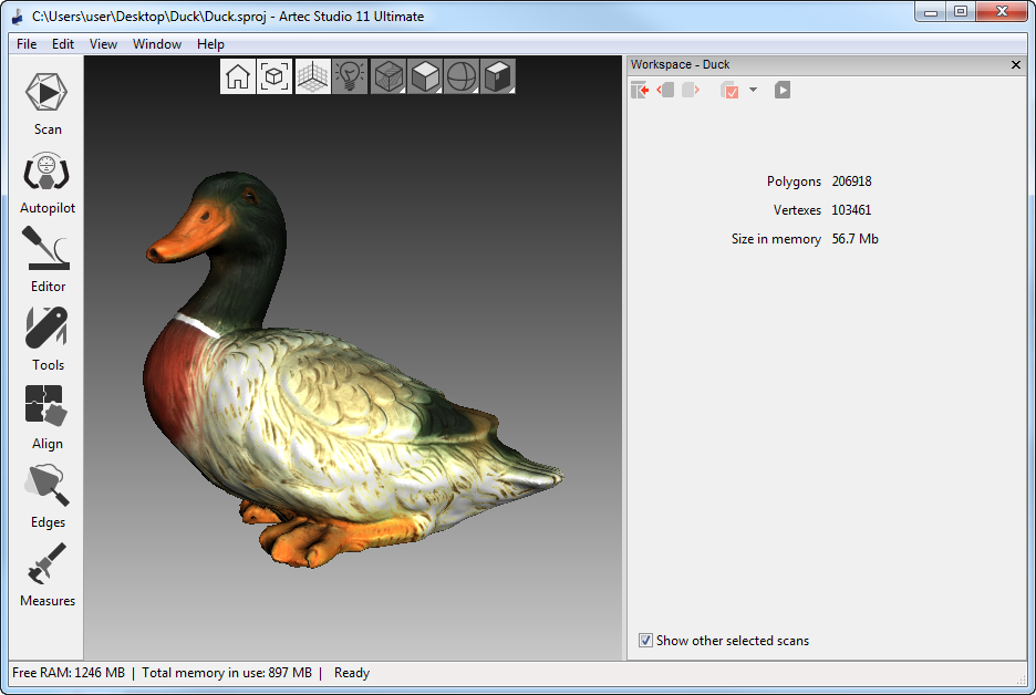
Figure 74. Single-frame scan (model) representation.
Revising Scans
As you begin building a 3D model, you should start by preprocessing your scans: remove unwanted frames, separate misaligned areas (if any) into separate scans and cut out unwanted objects from the scene.
You may, however, encounter the following problems:
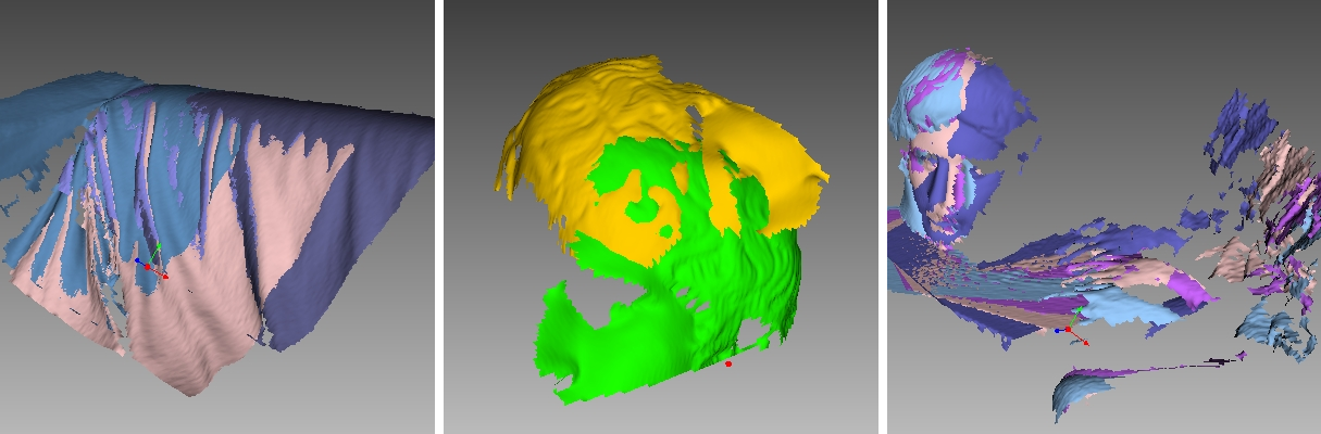
Figure 75. Possible scan errors.
- Misaligned frames (see Figure 75., left)—may occur because of small size, an insufficient number of geometrical features on the object or an insufficient number of polygons in a frame.
- Misaligned parts (see Figure 75., middle)—occurs when the real-time alignment algorithm incorrectly determines the position of the new frame relative to previous ones.
- Unwanted objects in the frame (see Figure 75., right).
A visual inspection of the frames can be very helpful in determining problematic areas. To perform a visual inspection, select the scan and view all the frames that it contains by holding Up Arrow or Down Arrow on the keyboard. This technique can easily detect misaligned frames.
See also
Removing Unwanted Frames
You must delete from your scans any misaligned frames as well as frames with an insufficient number of polygons. To do so, select the frames from the list and hit Delete.
Note
The system will not ask you for confirmation before performing this operation; it will delete data instantly once you hit Delete. You can restore deleted data by clicking the  (Undo) button.
Separating Scans
During the fine-alignment process, frames in certain scans may be misaligned. Sometimes it’s possible to divide the problematic scan into several scans, where each part is registered fairly well. In this case, divide the scan. To move some of the frames into a new scan, use the following procedure:
- Select in the Surface List panel the frames you want to move (see Selecting Frames).
- Click
RMBand select Move to new scan (Figure 73., right).
You can also fix alignment errors in another way: reset the current frame-transformation values and repeat the registration, making any appropriate changes to the settings.
Select the desired scan in the Workspace panel, click on it using RMB and select Reset transformations from the dropdown menu. Doing so will reset the computed positions of individual frames in the scan. A dialog will then appear, prompting you to confirm the operation.
To compute new positions, run the Rough serial registration and then Fine registration algorithms (see Fine Registration).
Editing Scans
To edit selected scans, open the Editor tools from the side panel. The  ,
,  ,
,  ,
,  ,
,  and
and  icons will appear alongside the icon bar in the 3D View window. These buttons correspond respectively to the Positioning, Transformation, Smoothing brush, Eraser, Defeature brush and Texture-healing brush tools.
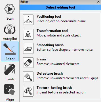
Figure 76. Editor panel.
Moving, Rotating and Scaling (Transformation Tool)
The Transformation tool allows you to move, rotate or scale objects in the 3D View window.
To access this tool, open the Editor panel and select Transformation tool by either clicking or hitting T. The panel will open, displaying three tabs that correspond to different modes for altering the object position in the global coordinate system. The name of the active mode appears at the bottom of the 3D View window.
- To enter translation mode,
click the Translate tab or hit
T. Three input fields will appear in the Editor panel showing the current origin coordinates (in millimeters) of the local coordinate system. The initial position of the local coordinate system will be in the center of the global one. To translate an object, do either of the following:- Enter the new coordinate values for the local system using the input fields in the Editor panel. To adjust the position only along a specific axis, first hit the corresponding
X,YorZkey. - Freely translate the object in the 3D View window by dragging the control square. Or translate the object along a specific axis by dragging only the necessary control arrow near the control square (see Figure 77.).
Note
Orienting the object may be easier if you first specify a new position for the origin of the local coordinate system: double-click on the desired surface point in the 3D View window.
- Enter the new coordinate values for the local system using the input fields in the Editor panel. To adjust the position only along a specific axis, first hit the corresponding

Figure 77. Translation control
- To enter rotation mode,
click the Rotate tab or hit
R. Three input fields containing the Euler-angle values will appear in the Editor panel. Initially, all values are set to zero. To rotate the object, do either of the following:- Enter the new angle values (in degrees) using the input fields in the Editor panel.
- Drag one of the three circles (see Figure 78.) to rotate the object. Hitting the key that corresponds the required axis (
X,YorZ) will hide the controls for the other axes.
Note
Orienting the object may be easier if you first specify a new position for the center of the local coordinate system: double-click on the desired surface point in the 3D View window.
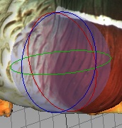
Figure 78. Rotation control
- To enter scaling mode,
click the Scale tab or hit
S. A single input field with the current scale value (1.000) will appear in the Editor panel. You have two options for scaling the object:- Enter the new scale value in the field.
- Drag the origin of the control (Figure 79.) or either of its round ends in the 3D View window.
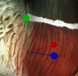
Figure 79. Scaling control
After altering the object using any of the methods described above, confirm or cancel your changes by clicking Apply or Cancel, respectively.
Each time you click Apply, Artec Studio will save the object position in the project history. Therefore, you can revert to the initial object position using the (Undo) button in the Workspace panel after you exit the Editor panel.
Placing Objects on Coordinate Plane (Positioning Tool)
You may need to place the model on one of the coordinate planes (e.g., for aesthetic reasons or when preparing the model for measurements, for capturing a screenshot, for exporting and so on). Instead of adjusting the model position using the Rotate and Translate modes of the Transformation tool, you can use the special Positioning tool. To do so, follow these steps below.
Tip
The Enable automatic base removal option may come in useful to position scans automatically after the scanning completes (see Base Removal: Erasing a Supporting Surface.)
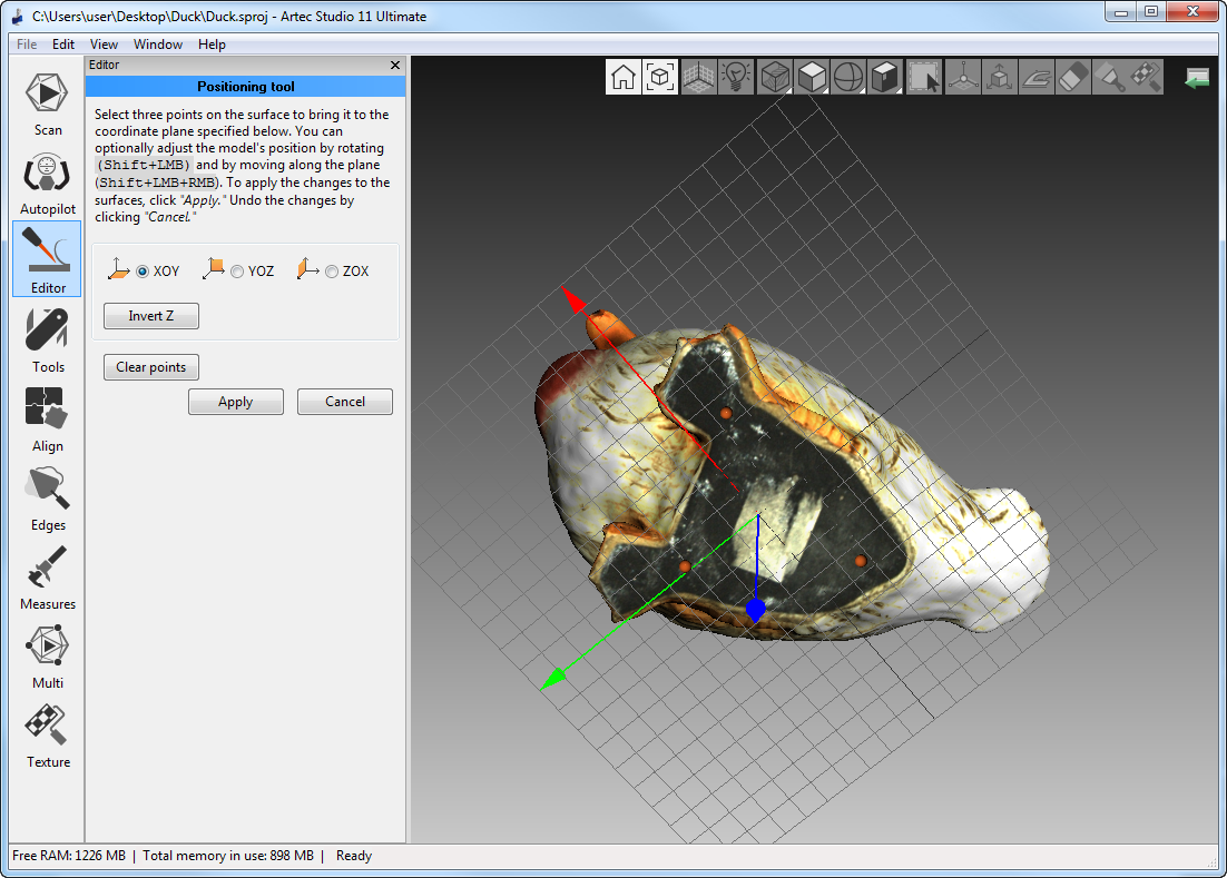
Figure 80. Positioning the model in the global coordinate system.
Open the Editor panel from the side toolbar and click either Positioning tool or the
 button in the upper part of the 3D View window, or hit
 P.Choose the coordinate plane in which you want to place the model by activating one of the following options: XOY, YOZ or ZOX. Note that you may skip this step and return to it after Step 3.
Use
LMBto specify at least three points on the surface; the plane will automatically pass through their center of mass (see Figure 80.). The following conditions will then apply:For each additional point you specify, Artec Studio rebuilds the plane. Click Clear points at any time to redefine the points.
Note
Three points determine a plane. When you’re dealing with nonplanar surfaces, however, three points may be insufficient. In that case, the more points you specify, the more precisely a plane will fit the surface.
In addition to the plane passing through the center of mass of the points you select, the coordinate origin will shift to that location as well.
The position of the coordinate origin is adjustable, as Step 5 describes.
Invert the direction of the coordinate axis, if desired, by clicking the Invert Z button for the XOY plane, Invert X for YOZ, or Invert Y for ZOX.
If appropriate, adjust the model’s position relative to the coordinate origin:
Shift + LMB—rotate the model around the axis that is currently normal to the planeShift + RMB—move the model along the plane in a fixed directionShift + LMB + RMB—move freely along the plane
Hit Apply to fix the model on a specified plane or Cancel if you are dissatisfied with the position.
Smoothing Brush
The Smoothing brush is a tool that you can employ selectively in specific areas without touching areas that require no alteration (for more information about automatic smoothing, consult Smoothing).
To use the Smoothing brush,
Select just one surface
Open the Editor panel, and click the
icon or hit S.Hit
Ctrl, an orange region will appear around the cursor in the 3D View window.Change brush size if necessary:
- Use either the
Ctrl + [andCtrl + ]shortcuts or - Use
Scroll wheel. - Enter a size (in millimeters) in the Brush size field.
- Alternatively, you can adjust the slider bar in the Smoothing brush panel.
- Use either the
Set the smoothing strength if necessary:
- Enter the desired value in the Smoothing strength field or
- Adjust the slider bar.
Hold
LMBand paint the surface region in order to smooth it. The tool will smooth the affected areas (see Figure 82., right).
Once you’re done, click the Apply or Cancel button.
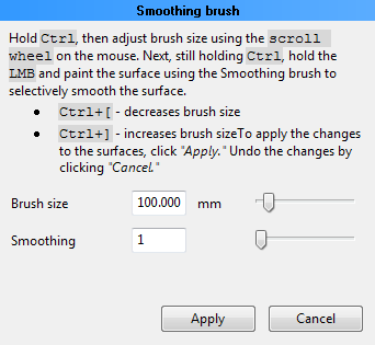
Figure 81. Smoothing brush panel.
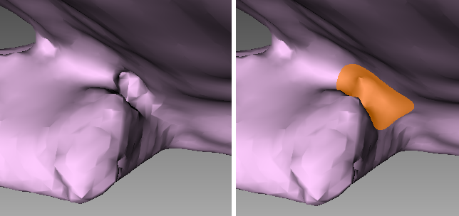
Figure 82. Before smoothing (left) and smoothing out a poorly captured area (right).
Erasing Portions of Scans
Nearly always, the scanning process will capture unwanted elements, such as walls, the operator’s hands, surfaces on which the object is located and other extraneous objects. This unwanted data can hinder postprocessing. To avoid this problem, we recommend eliminating these objects before processing. We designed several options to quickly and easily remove unwanted elements from the scene (see Figure 84.).
- 2D selection
- —is designed for deleting areas and elements of medium size.
- 3D selection
- —is useful for accurately cleaning small object areas.
- Rectangular selection
- —allows you to select large rectangular regions.
- Lasso selection
- —allows you to create a selection by freely outlining it with the cursor.
- Cutoff-plane selection
- —is a special mode for removing flat surfaces (table, floor or base) on which the object is resting. This mode uses a cutting plane that divides the scan into two parts: the first will remain and the second will be erased (see Figure 87.).
Tip
The Enable automatic base removal option deletes the supporting surface automatically after you close the Scan panel (see Base Removal: Erasing a Supporting Surface.)
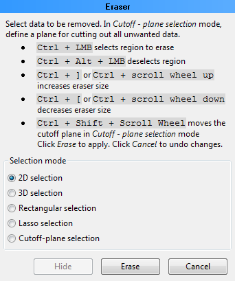
Figure 83. Eraser panel.
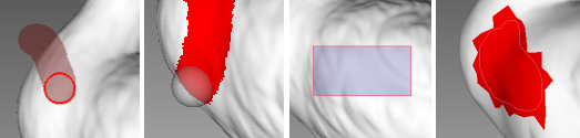
Figure 84. Various Eraser modes (from left to right): 2D, 3D, Rectangular, Lasso.
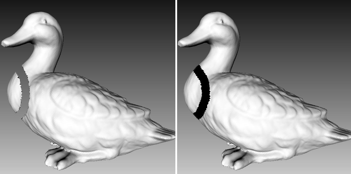
Figure 85. Select through in 2D Eraser: enabled on left and disabled on right.
Use the following general procedure to erase unwanted elements:
In the Workspace panel, select the scan you want to edit and open the Editor panel by clicking its icon in the side toolbar. Editor icons will appear alongside the existing ones in the 3D View toolbar.
If the scan is rendered with no texture, make sure its color is neither red nor any shade of red. Assigning non-red colors to the scan will help you easily identify the polygons you have selected for erasure. If necessary, change the scan’s color by clicking the colored square (
 ) near its name.
Open the Eraser tool by clicking
or by hitting E.Select the desired erasure mode (consult the list above).
Note
If you intend to use Cutoff-plane selection, make sure the Select through toggle is in the
 position in the 3D View window.
Mark the elements you want to erase. Hold down the
Ctrlkey and do any one of following, depending on the active mode:- 2D/3D selection—adjust the tool size (see Table 7.) and paint over the area using
LMB. - Rectangular selection—drag the cursor to select a rectangular region.
- Lasso selection—drag the cursor to freely outline an irregular region.
- Cutoff-plane selection—adjust the tool size (see the table) and paint over the flat area. Once you have released the mouse button, a plane will appear (see Figure 87.). If necessary, adjust the plane level by using
Scroll wheelwhile holding downCtrl+Shift.
- 2D/3D selection—adjust the tool size (see Table 7.) and paint over the area using
Click Erase to eliminate the area highlighted in red or to apply cutting plane.
| Purpose | Procedure |
|---|---|
| Deselect region | Reselect the region while holding down Ctrl+Alt |
| Undo operation | Hit Ctrl+Z or click |
| Adjust tool size | Use ] and [ keys or Scroll wheel while holding down Ctrl |
| Protect backface from erasure | Use Select through toggle: —backface is protected (see Figure 85., right); mandatory for Cutoff-plane selection —backface is affected (see Figure 85., left) —backface is affected (see Figure 85., left) |
| Reach difficult-to-access regions | Select (in the same way as for erasure) occluding polygons and click Hide |
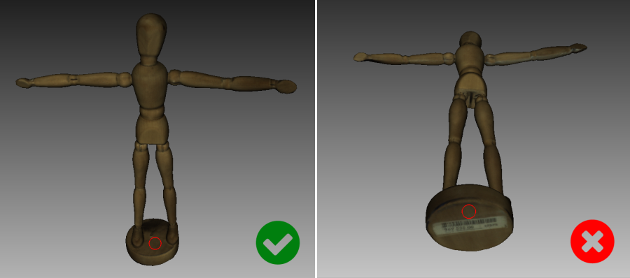
Figure 86. Selecting a flat region in the Cutoff-plane selection mode.
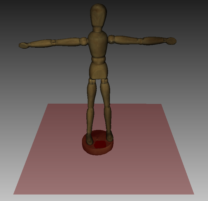
Figure 87. Cutting plane
Figure 88. Erasing results
Hiding Polygons When Using Eraser Tool
If polygons obstruct the region you want to erase, you can hide them. Before doing Step 5 of the procedure under Erasing Portions of Scans, do the following:
- Ensure the Select through toggle is in the position in the 3D View window.
- Mark the obstructing region using the technique described in Step 5 of the procedure.
- Click Hide to gain access to the obstructed region.
- Mark the region you want to erase.
Defeature Brush
Erasing certain geometrical imperfections often demands further processing of the resulting holes in the model. The Defeature brush combines functions of the Eraser and Hole filling tools and may boost your productivity. To use it, follow these steps:
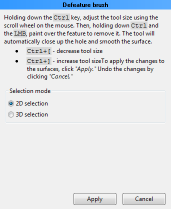
Figure 89. Defeature brush panel.
Select the surface in the Workspace panel. You can only choose one model or one frame from the scan.
Open the Editor panel using the side toolbar and click either Defeature brush or the
 button in the upper part of the 3D View window, or hit
 D.In the Editor panel, choose the selection type: 2D selection or 3D selection. The operating principle is the same as for the Eraser tool—that is, in 2D mode all surfaces throughout the model are affected (if
toggle is enabled), while in 3D mode the brush only works on the visible surface.Note
For most surfaces, results obtained in 2D mode with
toggle disabled will be approximately the same as those in 3D mode.Hit
Ctrlto activate the tool. Depending on the selection type, a red circle or an orange spot will appear in the 3D View window.While still holding down
Ctrl, adjust the spot size (see Figure 90., 4) or circle diameter (see Figure 90., 3) usingScroll wheelor the[and]keys. Their size should match the size of feature you want to remove.While still holding down
Ctrl, press and holdLMBand paint over the area you want to modify. A red stroke will appear. When you releaseLMB, the software will delete the feature, close up the hole and smooth the surface.If necessary, repeat Steps 3–6
Click Apply to implement all changes.
Note
If you are editing a textured model, don’t forget to enable the Render polygons without texture option in the View menu (see Rendering and Texturing Untextured Polygons) to display the processed surfaces. Note that the texture will disappear, but you can restore it through texture mapping (see Applying Texture).
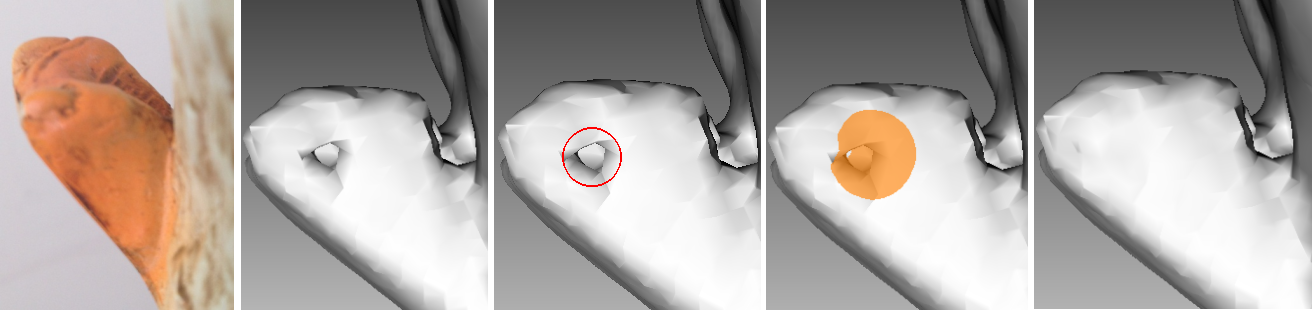
Figure 90. Defeature brush in action.
Fine Registration
Fine registration is an algorithm designed to automatically and precisely align captured frames. It starts once you complete scanning and close the Scan panel [1].
Note
Since the Fine registration algorithm runs automatically and uses the settings in the Tools panel, ensure that you have specified the proper (or, better, the default) values before you start scanning.
In a number of cases you can start the Fine registration algorithm manually using the Tools panel. To access a list of parameters, click the  button in the Fine registration section. The algorithm affects all scans marked with the icon in the Workspace panel (see Selecting Data for more information on scan selection), but it processes them separately.
| [1] | There is another post-scanning algorithm: automatic base removal (see Base Removal: Erasing a Supporting Surface.) |
From two to three parameters may be available. You can redefine either of them:
- registration_algorithm
is a type of registration algorithm
- Texture_and_Geometry
- takes both texture and geometry into account. If the scan lacks texture information, the algorithm will run on geometry only.
- Geometry
- uses geometry only. Unless your scan entirely lacks texture, we recommend avoiding this option.
- refine_serial
- is enabled by default for Geometry mode and is available as an option for Texture_and_Geometry mode. It represents the conventional fine serial-registration algorithm and registers in-series captured frames.
- loop_closure
- is an advanced algorithm that registers any frames not necessarily captured in series. Using any common regions in these frames, it compensates for cumulative error (see Figure 93.) caused by the peculiarities of handheld-3D-scanner movements. We highly recommend enabling this algorithm when you’re using Texture_and_Geometry mode.
Figures below illustrate how each algorithm works if launched independently. The call-out boxes in each figure show two frames from the same corner of the door: one captured at the beginning and one at the end of the scanning session. The captured data (see Figure 91.) has a cumulative error that is noticeable in the call-out box. The serial registration algorithm improves frames’ relative position (see Figure 92.), but misalignments remain. The loop-closure algorithm eliminates these misalignment completely (see Figure 93.).
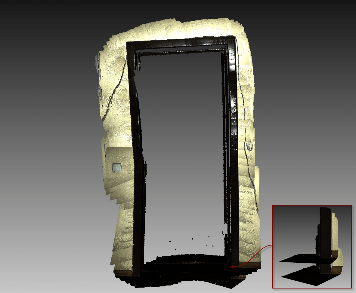
Figure 91. Rough data as is
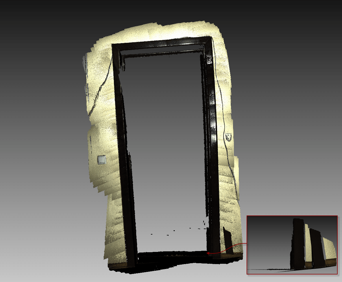
Figure 92. Serial-registration results
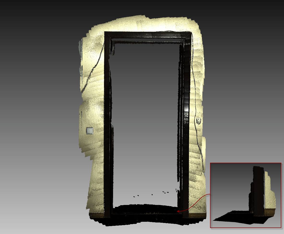
Figure 93. Loop-closure results
Scan Alignment
Although Artec Studio features continuous scanning, there may be some cases where the application lack sufficient information about the relative positions of multiple scans. To assemble all scans into a single whole, you must convert the data to a single coordinate system—that is, you must perform alignment using the Align tool.
Hint
If you find the coverage too long, you can refer to Auto-Alignment first. Take a glance at the Summary of Alignment Modes as well.
Selecting Scans for Alignment
In the Workspace panel, use the flag to mark all scans that you intend to work with. Once you click Align in the side panel; the marked scans will appear in the left panel in the same order as they appear in the Workspace panel. During the Align operation, Artec Studio divides the selected scans into two sets: aligned (registered) scans and unaligned scans. The first set initially contains only one scan (the first one in the list), which is highlighted in blue. Its name appears in bold and uses the same color icon ( ). Auto-Alignment, however, may produce several groups of aligned scans.
The user’s task is to align all scans to those that are already registered and to “assemble a model”. In general, the procedure includes the following steps:
Click the required tab in the Align panel.
Select one scan from the unregistered group in the Align panel. The name of unregistered scan appears in a regular typeface. When selected, the unregistered scan is marked by the green icon
 . You can select several scans using either of the following methods:
- Press and hold down the
Ctrlkey, and then click each scan that you want to select - Click the first item, press and hold down the
Shiftkey, and then click the last item.
- Press and hold down the
If necessary, specify point pairs (for two scans) or sets of points (for more than two scans) and click the desired alignment-command button (Auto-Alignment is the most recommended one). The command affects all scans selected in the Align panel plus the first one (
).
Since each mode varies in its effects, see the details in the corresponding subsections for more information. Note that you can use either one mode or a series of modes (see comparison table in Summary of Alignment Modes): drag alignment, rigid alignment with and without point specification, automatic rigid alignment, and alignment with surface deformations.
Changing Scan Status
If you have already aligned several scans, you should move them to the registered group. Select them in the Align panel using LMB. Next, click RMB on the name of any scan and select the Mark as registered option from the dropdown menu, or just double-click its name in the list. At this point, Artec Studio will treat registered scans as one, so you cannot move them independently.
If you accidentally mark a scan as aligned, remove it from the registered group by selecting the Mark as unregistered item from the dropdown menu, or just double-click it.
Displaying Scans in 3D View
Scans selected in the Align panel appear in the 3D View window. Keys 1, 2 and 3 switch among scans in the 3D View window:
1- shows aligned scans and groups
2- shows scans that are currently under alignment
3- shows all scans
Navigation in align mode is similar to navigation in the 3D View window:
- Rotate
- hold
LMBand move mouse - Zoom in/out
- use
Scroll wheel, or holdRMBand move mouse - Move
- hold
LMBandRMBsimultaneously, or hold the middle button, and move mouse
Summary of Alignment Modes
The table below provides basic information on the various alignment modes (see Scan Alignment).
- Scan type lists which scans you can use in a particular mode.
- Scans per operation is the number of scans required to use a particular mode.
- Markers in set prescribes how many markers (points) you can map in one point set. Some modes require point (marker) sets, but some don’t.
- “—” means that markers are unnecessary.
- “0 or 2” means point specification is optional and, if you do specify them, only marker pairs are allowed.
- “At least 1” means you can specify an unlimited number of markers in one set.
| Mode | Scan Types | Scans per Operation | Markers in Set | Notes |
|---|---|---|---|---|
| Rigid (markers) | Any | 2 | 2 | Considers only coordinates, not geometry |
| Rigid (meshes) | Any | 2 | 0 or 2 | Considers geometric features |
| Rigid (texture) | Multiframe with poor geometry | 2 | 0 or 2 | High resource consumption |
| Rigid (auto) | Any | Any number | — | Works if surface is well textured |
| “Drag” | Any | 2 | — | Interactive |
| Nonrigid | Models | Any number | 0 or 2 | Deforms surfaces and textures; pre-alignment required |
| Complex | Any | 1 (at least 2 for models) | At least 1 | Precise and flexible |
Drag Alignment
Drag alignment is always available, regardless of which tab is active in the Align panel. This mode allows you to align scans by manually dragging them in the 3D View window.
Owing to the low accuracy of this approach, however, you can optionally use it for preliminary alignment before running more-accurate modes.
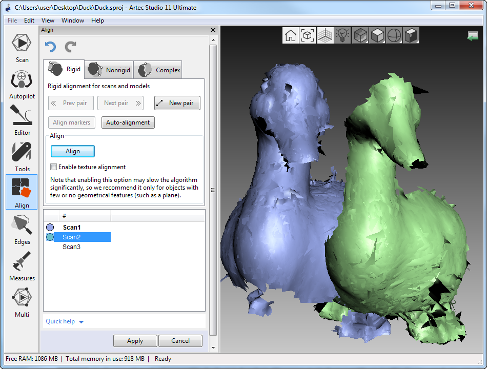
Figure 94. Dragging a scan
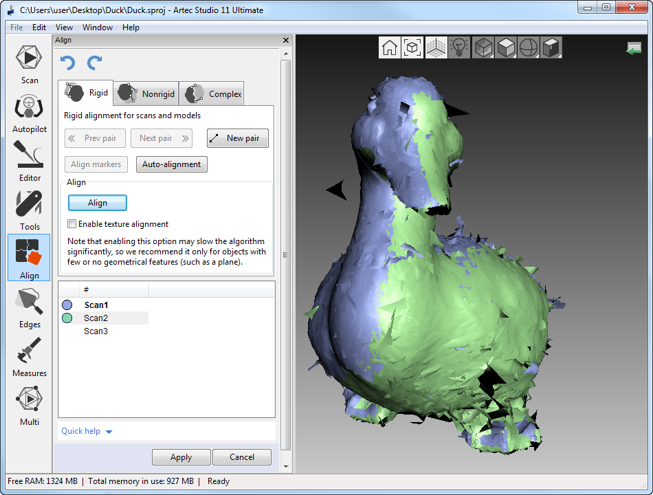
Figure 95. “Drag” alignment result
- Select the scan you want to align, keeping in mind the recommendation at the beginning of Scan Alignment. Artec Studio allows you to select multiple scans, but note that it will align them with the registered scans as a single unit.
- Holding down the
Shiftkey and one mouse button, move and rotate the scan you’re aligning (a green one) close to the registered scan (a blue one ). Scan Alignment provides a list of allowed movements and corresponding buttons. - To confirm the alignment, release the mouse button(s) and the
Shiftkey, then click Apply. Note carefully that any scans you are registering won’t automatically move to the registered set (see Figure 95.). You can do so manually as the beginning of Scan Alignment describes. - If you have several scans to align, repeat these steps for each one individually.
Auto-Alignment
Rigid alignment is a universal mode suitable for aligning most scans. Auto-alignment is the easiest approach, however. The advantages of this latter mode include the ability to align several scans at once and avoid the need to specify points; the only disadvantage is minimum requirements for the size of the overlapping areas in the scans you’re aligning.
To perform auto-alignment, follow these steps:
- Make sure the Rigid tab is selected (see Figure 97.).
- Select all the scans by using either
CtrlorShift, as the Scan Alignment section mentions. - Click Auto-alignment. Ideally, Artec Studio aligns all the scans and marks them using the icon. It may, however, mark scans as registered even though the 3D surfaces failed to join properly.
Important
Auto-alignment may be unsuccessful if the scans have small overlapping area.
Auto-alignment may produce the following results:
- Aligned scans, marked with the icon (basic group of registered scans)
- Unregistered scans, marked with the icon
- One group (
 ) or several groups (
 ,
,  ) of registered scans. Scans forming this group failed to align with the basic registered group (), although they succeeded in aligning with each other.
We recommend resolving issues with unregistered scans or registered groups by aligning them manually as Manual Rigid Alignment Using Point Specification describes. Other methods may also help.
Managing Groups and Scans
You can perform the following actions on the scans from the list in the Align panel (right-click on the item to open the context menu):
- Mark as registered
- Only available for single unregistered scans ( → )
- Mark as unregistered
- Use this command to discard the alignment state of a particular scan (unavailable for scans)
- Select group
- Highlights the respective group (, , and so on)
- Mark group as registered
- Converts all scans from the group into the basic registered group ( → )
Manual Rigid Alignment Without Specifying Points
You can perform rigid alignment either with or without specifying points. If the scans are close to each other in distance (e.g., after “drag” alignment), or if they have a large overlapping area or rich texture, you can skip the task of point specification when aligning them.
Perform the following steps:
- Make sure the Rigid tab is selected (see Figure 97.).
- Select the scan you want to align, as the beginning of Scan Alignment describes.
- Click Align. The result should be as Figure 99. depicts. If you are dissatisfied with this result, click
 and follow the recommendations in Manual Rigid Alignment Using Point Specification.
 - Select another scan from the list of unregistered scans and repeat the above procedure.
- Click Apply to confirm your alignment results or Cancel to reject them.
Texture Alignment
If the object was scanned with texture, the texture-alignment feature may ease the alignment process. It uses texture-image characteristics of scanned objects and greatly decreases the possibility of incorrect alignment. This feature also helps to align objects with few or no geometrical features, such as round or flat objects with no corners. If an object has rich, nonrepetitive geometry, however, we recommend disabling texture alignment to reduce the algorithm’s running time. Also keep in mind that texture alignment will be useless if the object texture is monochrome.
To enable texture alignment, select the Enable texture alignment checkbox at the bottom of the Align panel just before you perform Step 3 of the procedure above.
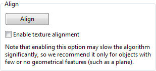
Figure 96. Checkbox for texture alignment.
Note
Texture alignment is a resource-intensive algorithm that slows down the alignment process. We recommend using it only in cases where the object’s geometrical features are insufficient.
Specifying Points and Editing Their Positions
Before considering how to align scans using points, it is helpful to highlight point-pair specification. The alignment algorithm uses pairs of point, or point sets in “Complex alignment” mode (Complex Alignment), to detect scan areas that should be brought close together.
To do point alignment, create several point pairs. To create one pair, mark one point on the aligned scan and then mark another one on the unaligned scan. Ensure that in each case the points for a given pair match a corresponding point on the surface of a real object; note, however, that high matching accuracy is unnecessary, since Artec Studio only uses the pairs to gain a rough approximation before performing precise registration. In the Complex mode, you can create a set of points (instead of just a pair), i.e. you can simultaneously specify more than two points in one or several unregistered scans and only one in the registered scan. All these points are connected by polylines and form a set.
When specifying points in the Rigid and Nonrigid modes, the application automatically creates pairs. Having specified one pair, you can immediately create the next one. In Complex mode you must confirm set creation by hitting Space or by clicking New set from the left panel, because the set may comprise multiple points (see Figure 98. and Figure 104.).
You can toggle between the point pairs (sets) by hitting Space and Backspace, or by clicking RMB in the 3D View window and selecting the relevant options from the menu. You can also relocate points in the pair (set). Hover the mouse cursor over the point until the pair (set) is highlighted in white, then drag the point to the proper position using LMB, or select the pair (set) and specify a new position using LMB. To confirm your actions and deselect the pair (set), hit Space. You can also remove either a pair (set) or one of its individual points: click on the point using RMB and choose the appropriate command from the menu. Alternatively, you can use Del to remove the selected pair (set).
Manual Rigid Alignment Using Point Specification
We advise using this mode when scans are located at a significant distance from each other.
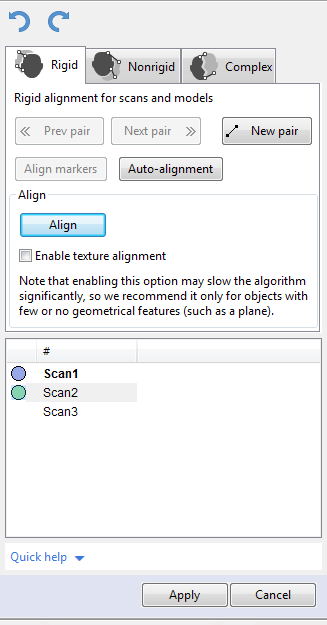
Figure 97. Align panel: Rigid tab.
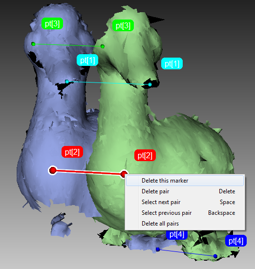
Figure 98. Creation of point pair.
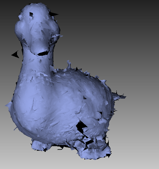
Figure 99. Alignment result.
To use this approach, follow these steps:
- Make sure the Rigid tab is selected (see Figure 97.).
- Select the scan you want to align, as the beginning of Scan Alignment describes.
- Specify several point pairs (Figure 98.), keeping in mind the recommendations from Specifying Points and Editing Their Positions.
- Click Align markers. This mode takes into account only the coordinates of specified points and tries to reduce the distance between the markers for each pair.
- Carry out Steps 3–5 of the procedure in Manual Rigid Alignment Without Specifying Points.
Nonrigid Alignment
Whereas rigid alignment can only perform such transformations as translation and rotation, the nonrigid algorithm can deform 3D data. This algorithm is intended to process so-called nonrigid objects: objects whose shapes have changed during the scan (e.g., models of animals or humans—see Figure 101., left). Keep in mind that the surface Artec Studio produces as a result of the deformation may differ from the surface of the actual object.
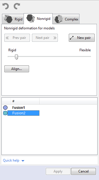
Figure 100. Align panel: Nonrigid tab.
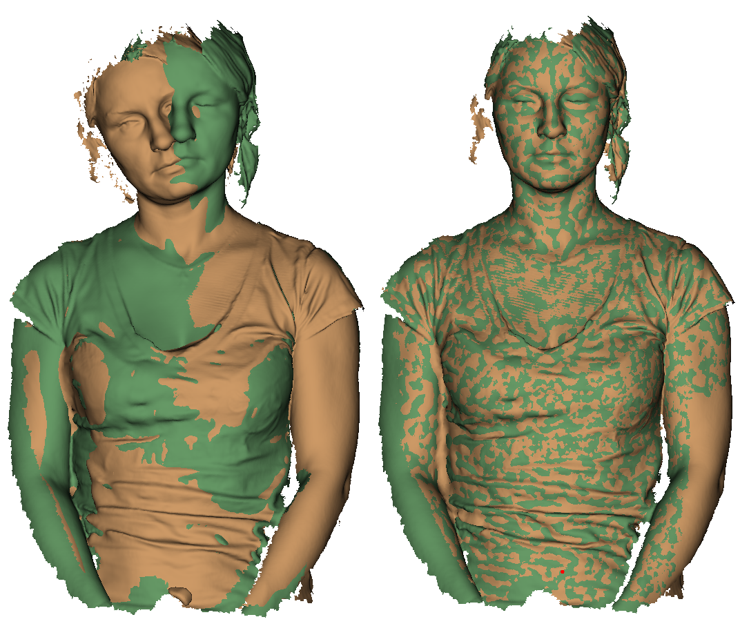
Figure 101. Two models after rigid (left) and nonrigid alignment (right).
Note
Nonrigid alignment works on models only. Thus, before you run it, prepare models by fusing the source scans. It is also necessary to first align models in rigid mode (see Manual Rigid Alignment Without Specifying Points, Auto-Alignment or Manual Rigid Alignment Using Point Specification).
To run the nonrigid alignment, follow these steps:
Make sure the Nonrigid tab is selected (see Figure 100.).
Select the models you want to align, as the beginning of Scan Alignment describes.
If the models differ significantly from each other, we suggest that you specify several point pairs, keeping in mind the recommendations in Specifying Points and Editing Their Positions.
Where necessary, adjust the deformation degree using the flexibility slider. The greater the flexibility value (i.e., the more “flexible” the deformation), the longer the computation will take.
Warning
Avoid extreme Flexibility values. Applying very large values may result in major surface distortions and may slow down the algorithm. Extremely low values, on the other hand, barely deform surface and often fail to produce the expected nonrigid-alignment results.
Click Align.... The algorithm will align models by deforming one of the model (see Figure 101., right). If you are dissatisfied with the alignment results, click
and specify additional point pairs, or reposition the current pairs.Select another model from the unregistered set and repeat the steps above.
Click Apply to confirm your alignment results or Cancel to reject them.
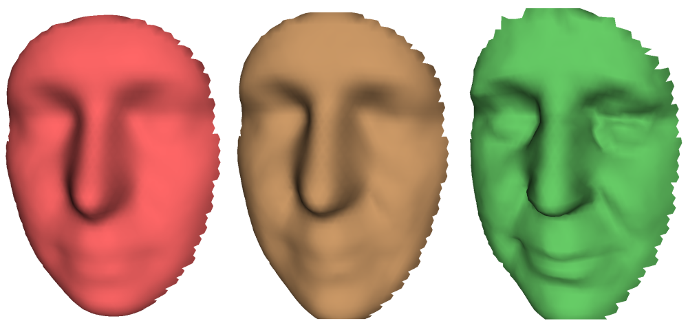
Figure 102. Flexibility slider in action: original model (left), nonrigidly aligned model with low Flexibility value (middle) and with high value (right).
Note
This version of Artec Studio does not support texture mapping on nonrigidly aligned models.
Complex Alignment
Complex alignment allows you to align not only scan to scan, but surface to surface within a given scan (see the mode comparison in Summary of Alignment Modes). Relative to other modes, this one supports multipoint-set definition—that is, you can link more than two points. It’s useful for aligning scans obtained during circular movements of the 3D scanner in cases where fine registration with the loop_closure option enabled fails to align them. To run the Complex alignment, perform the following steps:
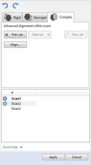
Figure 103. Align panel: Complex tab.
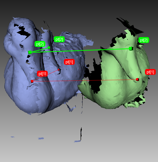
Figure 104. Before alignment: two point-set added.
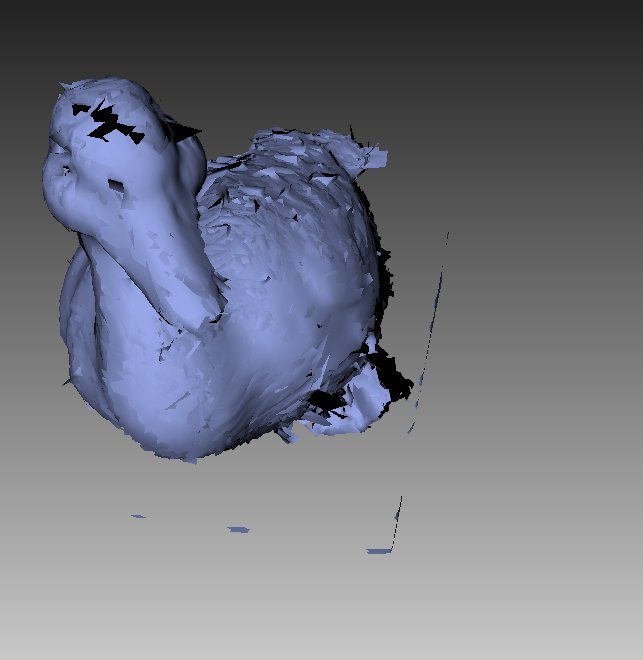
Figure 105. Alignment result.
- Make sure the Complex tab is selected (see Figure 103.).
- Select the scans you want to align, as the beginning of Scan Alignment describes. This mode allows you to work even with just one registered () scan.
- Specify one or more point sets on the scan surface (see Figure 104.), keeping in mind the recommendations in Specifying Points and Editing Their Positions.
- Click Align... to run the alignment with your specified constraints (Figure 105. shows example results). If you are dissatisfied with the alignment results, click and specify additional point sets, or reposition the current sets. To redo an operation that you have undone, click
 .
. - Click Apply to confirm your alignment results or Cancel to reject them.
Global Registration
Once you have aligned all your scans, proceed to the next stage: global registration. The global-registration algorithm converts all one-frame surfaces to a single coordinate system using information on the mutual position of each surface pair. To do so, it selects a set of special geometry points on each frame, followed by a search for pair matches between points on different frames. To perform correctly, the algorithm requires an initial approximation, which a user ensures in the course of the Align operation.
Note
Global registration is a resource-intensive operation. Processing of large data sets may take a long time and require a large amount of RAM.
To launch the algorithm, select all aligned scans in the Workspace panel. Next, open the Tools panel and locate the Global registration section. Click Apply.
Global-Registration Parameters
- registration_algorithm
- the type of algorithm that will perform scan registration. If an object has rich texture and poor geometry, consider using the Texture_and_Geometry option. For objects with rich geometry, you can choose Geometry mode to increase the registration speed.
- minimal_distance
- the minimum distance between adjoining feature points on the object (in millimeters).
- iterations
- the number of iterations of the global optimization algorithm. Optimization is a part of the global-registration algorithm.
Possible Global-Registration Errors
- After the global-registration algorithm finishes, the frames are in disarray (see Figure 106., left) or the frame positions are unchanged. This error occurs because the application is configured for a different scanner type than the one that captured the data. Change the device type in the application settings (see Algorithm Settings).
- The algorithm has completed successfully, but a gap exists between two or more scans (see Figure 106., right). Select just these scans in the Workspace panel and run the global-registration algorithm. If the scans have drawn closer to each other but have failed to align after the algorithm finishes, increase the number of iterations and rerun the algorithm. Repeat this process until you achieve full alignment, then run global registration once again for all data. If you are unable to align several problematic scans, try aligning just two of them, then gradually increase the number of scans until all of them are aligned.
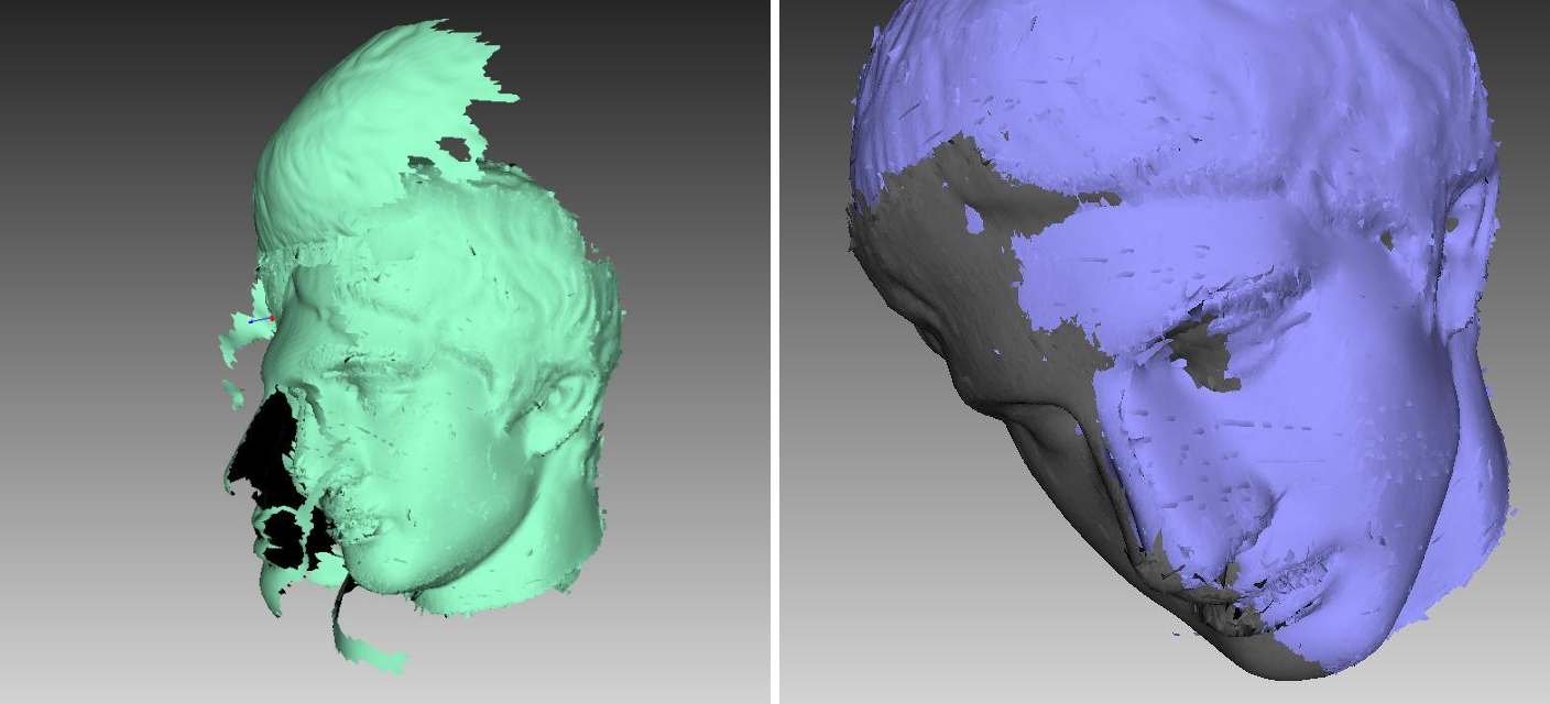
Figure 106. Global-registration errors: wrong settings on left and gap between scans on right.
Outlier Removal
During the scanning process, so-called outliers may appear in the scene. Outliers are small surfaces unconnected to the main surfaces. They require removal because they may spoil the model or produce unwanted fragments. Artec Studio provides two ways to remove outliers: erase them before fusion (preventive approach) or after fusion (“furthering” approach—see Small-Object Filter). We advise using the former approach because it decreases the possibility of improper fusion by preventing noisy features from attaching to the main surface.
This outlier-removal approach is based on a statistical algorithm that calculates for every surface point the mean distances between that point and a certain number of neighboring points, as well as the standard deviation of these distances. All points whose mean distances are greater than an interval defined by the global-distances mean and standard deviation are then classified as outliers and removed from the scene.
For better results, we recommend running global registration before starting the algorithm. If you begin Outlier removal before doing so, a dialog will appear prompting you to perform global registration.
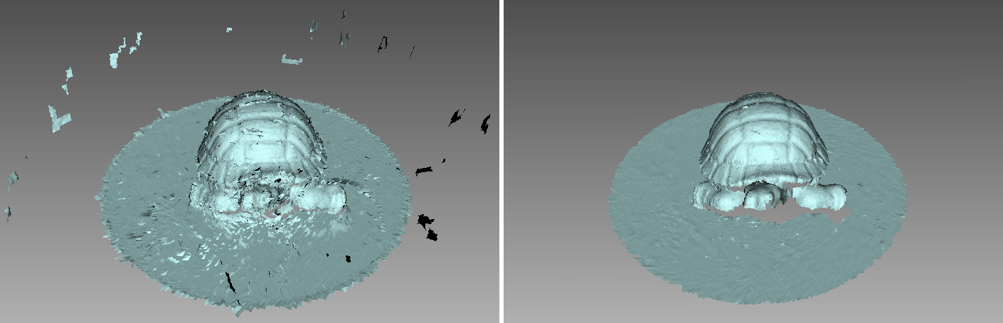
Figure 107. Outlier removal: before and after.
In most cases, none of the parameters accessible through the button requires adjustment. But if necessary, you can change the values of these parameters:
- std_dev_mul_threshold
a standard-deviation multiplier. We recommend choosing the value for this parameter according to the following guidelines:
2: for noisier surfaces 3: for less noisy surfaces - resolution
- should be set equal to the resolution of the Fusion process that you expect to run later.
Click Apply to run Outlier removal.
Fusion
Fusion is a process that creates a polygonal 3D model. It effectively melts and solidifies the captured and processed frames. Fusion is the most interesting part of the processing task because a polygonal 3D model is what most people expect to see when performing a 3D scan. To this end, you can use one of the following algorithms, each of which has a self-explanatory name (see also the summary in Table 9.):
- Fast fusion produces quick results.
- Smooth fusion is good for scanning the human body because of its ability to compensate for slight movements by the person you’re scanning.
- Sharp fusion perfectly reconstructs fine features and is suited to both industrial objects and human bodies. It is the only mode that allows you to use all the capabilities of a Artec Spider scanner.
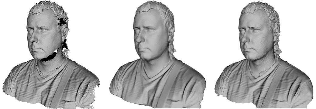
Figure 108. Models of a human subject obtained using various algorithms: Fast fusion (left), Smooth fusion (middle) and Sharp fusion (right).
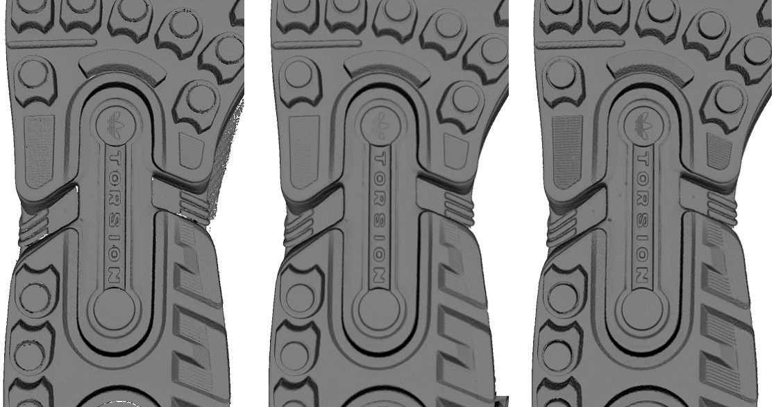
Figure 109. Models of a shoe sole obtained using various algorithms: Fast fusion (left), Smooth fusion (middle) and Sharp fusion (right).
| Fast Fusion | Smooth Fusion | Sharp Fusion | |
|---|---|---|---|
| Usage | Fast results for large data sets; also for measurements | Large, noisy data sets with patchy missing regions; scans of moving objects | Scans from Artec Spider; scans having regions with fine details and sharp edges |
| EVA | resolution no less than 0.4 | ||
| Spider | resolution no less than 0.1 | ||
| L | resolution no less than 1.5 | ||
| Fill_holes | Not applicable | Available | |
| Features | Resulting surfaces are relatively noisy. Offers an additional parameter, radius | Smoother results. Can compensate for slight movements, but not recommended for accurate measurements. Relatively slow. | Higher level of detail. Faster than Smooth fusion, but may intensify existing noise. |
To obtain a model:
- Make sure the scans you intend to fuse have passed Global registration.
- Select the scans in the Workspace panel using .
- Enter the Tools panel.
- Select the necessary mode; optionally, specify parameter values.
- Click Apply.
- View the model in the 3D View window and in the Workspace panel once the algorithm finishes. The model name will match the algorithm name.
The fusion algorithms use the following parameters:
- resolution
- —the step of the grid (in millimeters) that the algorithm uses to reconstruct a polygonal model. In other words, this parameter defines the mean distance between two points in a model. The lower the resolution value, the sharper the shape. When specifying values, keep in mind the default values and lower limits in Table 9..
- radius
- —only for Fast fusion, a multiplier or integer factor that defines the surrounding space that the algorithm takes into consideration when adding each new minimum spatial unit. Note that the size of the spatial unit remains unchanged and is equal to the resolution value; the actual search radius is the product of resolution and radius.
- Fill_holes
—instructs the algorithm to fill holes in the mesh being reconstructed; option unavailable for Fast fusion. The methods for filling the holes are as follows:
- By_radius
- —fills all holes with radius less than or equal to the specified value in the max_hole_radius text box (in millimeters)
- Watertight
- —automatically fills all holes in the mesh
- Manually
- —prompts you to fill holes manually in the Edges panel, which opens automatically
- remove_targets
- —allows you to erase small embossments from surfaces on which targets are placed (see Target-Assisted Scanning). Parameter can assume either the On or Off value; unavailable for Fast fusion.
Fusion-Algorithm Errors
Occasionally, defects appear in the 3D model after fusion; some are correctable by creating additional scans, whereas others are correctable by using the model-processing tools described in the next section.
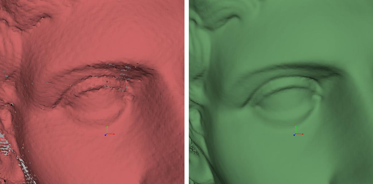
Figure 110. Surface noise caused by insufficient data (left) and improved model after adding one more scan (right).
Errors that can be corrected by capturing additional scans include low-amplitude noise on the surface (see Figure 110., left). Normally, this error indicates that the affected area has a small number of frames. The number of frames needed to eliminate the noise depends on the reflective properties of the object’s surface. To correct the error, you need one more scan to cover the noisy area (see Figure 110., right).
Sometimes the cause of noise is an insufficient number of scanning angles. Areas captured at a larger angle have more noise than areas captured at a direct angle (i.e., 90 degrees). You can correct this error by scanning the area again using a better angle.
When the scanning conditions or the object features are such that you are unable to capture additional data, you can correct errors using the Edges (see Filling Holes and Smoothing Edges) or Smoothing (Smoothing) tools. If such errors are frequent, reduce the speed at which you move the scanner around the object, or increase the capture rate (see Decreasing Scanning Speed).
Editing Models
The resulting fusion model may contain surface defects due to scanning or registration errors. Artec Studio provides a number of tools to correct such errors:
- Repair
- —corrects the model’s triangulation errors
- Small-object filter
- —removes small objects located near the model surface
- Edges
- —semiautomatically fills holes and smooths the model edges
- Hole filling
- —fills holes in the model automatically
- Smoothing
- —filters low-amplitude noise over the whole model
- Smoothing brush
- —enables manual smoothing of the surface areas with the most noise
- Mesh simplification
- —reduces the number of polygons in a model while minimizing lost accuracy
- Remesh
- —creates isotropic mesh while keeping the processed mesh as close to the original as possible
Each algorithm processes all scans selected in the Workspace panel and replaces the original data with the results. If the algorithm is unsuccessful, you can restore the original data by clicking (Undo) in the Workspace panel.
Correcting Triangulation Errors
Some algorithms may introduce triangulation errors into the resulting model. These errors include the following:
- Unattached vertices
- —points that are not vertices of any of the triangles
- Vertices with identical coordinates
- —vertices that have the same coordinates
- Faces containing invalid vertices
- —triangles that point to nonexistent vertices
- Singular faces
- —triangles for which at least two of the three vertices coincide.
- Faces with equal signature
- —faces with fully coinciding sets of vertices
- Edges incident to three or more faces
- —edges that are adjacent to three or more faces
- Faces with wrong orientation
- —faces whose normals point in a direction opposite to those of the adjoining faces
To correct these errors, mark a model in the Workspace panel by using the flag and hit Ctrl + R or select the menu command. If the algorithm detects no triangulation errors, Artec Studio will notify you that it has found no defects. Otherwise, the Repair panel will open, displaying the above-mentioned list of defects to be corrected.
Next to the names of the defects, a column will appear stating the number of defects of a certain type found in the model. You can select all defects by pressing View all. Doing so will display in the model all the defective vertices and triangles using colored points.
You can disable display of any particular defect type by removing the icon next to the corresponding name, or disable them all by clicking View none. To correct the defects, click Repair all. Clicking the Apply button accepts the changes.
Small-Object Filter
If you forgot to erase outliers before fusion (see Outlier Removal), Artec Studio may solidify and preserve them in the scene as small, distant fragments.
You can effectively remove these remaining outliers by using a filtering algorithm.
To remove these artifacts, select in the Workspace panel only the model you are currently editing, then open the Tools panel. Click Apply next to Small-object filter to run the algorithm (see Figure 111.).
A window containing algorithm settings will appear when you click . You can adjust the following parameters:
- mode
- —the Leave_biggest_objects option from the dropdown menu instructs the algorithm to erase all objects except the one with the most polygons; Filter_by_threshold erases from the scene all objects whose number of polygons is less than the amount specified in the threshold parameter.
- threshold
- —the maximum number of polygons for Filter_by_threshold.
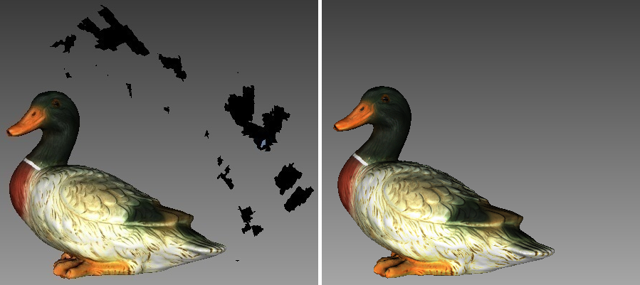
Figure 111. Filtering of scene outliers: before (left) and after (right).
Filling Holes and Smoothing Edges
Sometimes the shape of an object or the scanning conditions prevent you from properly capturing of all parts of the scene. As a result, the fused 3D model will have holes. In such instances, you can use the hole-filling tool to interpolate the surface.
To start analyzing and correcting the model,
Select the model and click Edges from the side panel. The new panel has two tabs: Edges and Holes, each of which contains a list of holes detected on the surface. These defects are sorted by their perimeter length.
Select a hole, Artec Studio will highlight the corresponding edge in the 3D View window.
Note
If the Move camera to selection option is checked, the model will automatically rotate to display the selected edge. By default, the camera moves smoothly from one edge to another when switching between edges. If the model is large, however, this movement may take too long. To expedite the switch, clear the Animate camera checkbox.
To select edges for correction,
- Mark the checkbox next to each one you wish to correct. These edges will be highlighted in red in the 3D View window (see Figure 112.).
- Use the Select all and Deselect all buttons in the panel to select or clear all selections, respectively.
- You can also select edges right on the model. To do so, rotate the model to make the edge visible in the 3D View window. Then click
LMBto select it.
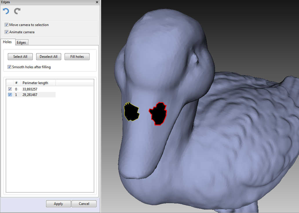
Figure 112. Two holes marked for correction.
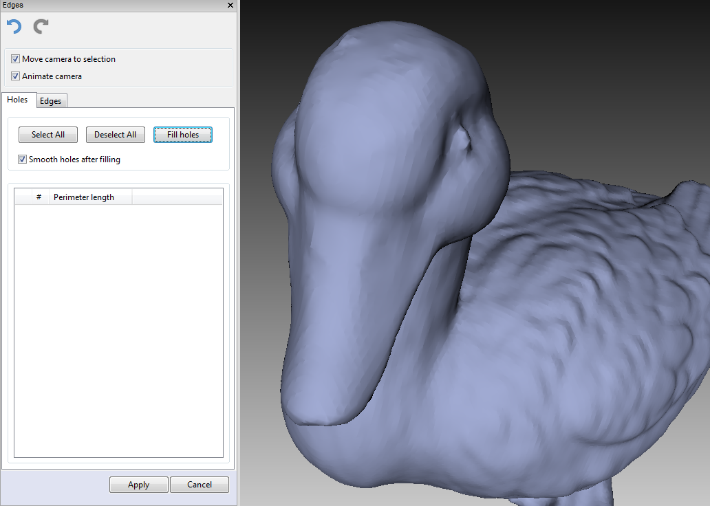
Figure 113. Result from running the Fill holes algorithm.
Under the Holes Tab, you can enable an option that automatically smooths the holes after filling them by checking the Smooth holes after filling box (see also Smoothing).
Under the Edges Tab, use the Strength slider to control the edge-smoothing intensity. Also, you can use this tab to smooth part of the edge instead of the whole one. To do so, rotate the model to make the edge visible and mark it in the list as “processing required.”
Next, hold down LMB and move the mouse over the edge to drag apart the ends of the profile to the desired position (see Figure 114.).
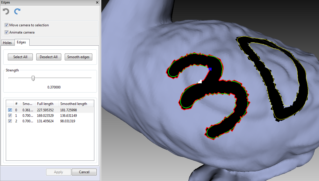
Figure 114. Boundary selection for edge smoothing
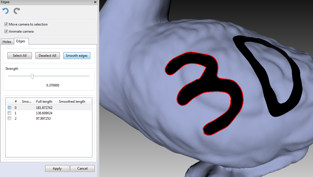
Figure 115. Edge-smoothing algorithm results.
After you have selected all the edges or the holes you want to fix, click Fill holes or Smooth edges. Artec Studio will repair the model. If the results are satisfactory, click Apply to confirm them; otherwise, you can always use the button to cancel any changes.
If you try to exit the Edges mode without accepting changes, the software will ask you for confirmation.
Automatic Hole Filling
To quickly and automatically fill holes, use the Hole filling algorithm in the Tools panel. It employs the same edges as the Edges tool, processing only those holes with parameters that correspond to the one user-adjustable setting, which you can access through the button:
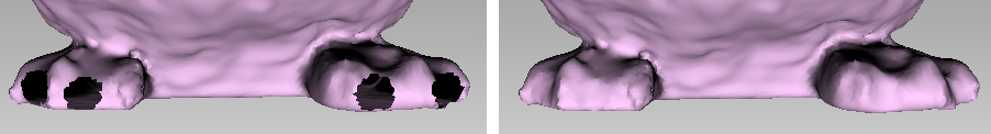
Figure 116. Hole-filling algorithm: original model on left, processed on right.
- max_hole_len
- maximum length of the hole perimeter in millimeters. The algorithm only processes holes with perimeters below this threshold.
Smoothing
The smoothing algorithm evens out noisy areas in the 3D model. Artec Studio provides two such tools: automatic smoothing of the entire model and manual smoothing of specific areas identified using a brush (see Smoothing Brush).
To run the automatic smoothing algorithm, open the Tools panel and select Smoothing. You need only set one parameter:
- steps
- —the number of algorithm iterations to be performed
Mesh Simplification
The mesh produced after fusion may be less than optimal for some applications because it will contain a large number of polygons. This complexity will increase the amount of memory the model occupies, hindering further processing. To optimize the model size while retaining accuracy, use the Mesh simplification algorithm.
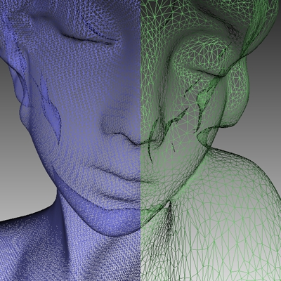
Figure 117. Mesh simplification: original mesh on the left, optimized mesh on the right.
Select the model and open the Tools panel. You can choose from two algorithms.
Conventional Algorithm
Open the dropdown algorithm settings by clicking the button next to Mesh simplification.
Select the appropriate processing method (determined by the stop_condition):
- Accuracy
- —optimize model to a predetermined accuracy: the error parameter defines the optimized model’s maximum allowable deviation (in millimeters) from the original model. When the algorithm reaches this value, the optimization stops.
- Remesh
- —perform simple mesh optimization, removing triangles whose edge lengths are less than the remesh_edge_thr value (in millimeters).
- Triangle_quantity
—simplify the model by targeting the number of triangles specified in the tri_num parameter. The algorithm minimizes the resulting model’s deviation from the original model, but the final deviation value will remain unknown until processing concludes. Use this method when you know how many triangles the resulting model should have.
Note
To determine the number of triangles, double-click the appropriate model from the list in the Workspace panel (see Figure 74.).
- UV_Triangle_quantity
- —similar to the Triangle_quantity algorithm, but intended for meshes with textures mapped by the Atlas method (see Applying Texture). This approach not only simplifies the polygon grid, reducing the number of triangles, but it preserves texture.
- UV_Vertex_quantity
- —simplify a textured model by targeting the number of vertices specified in the vrt_num parameter.
The three first algorithms in the list above have additional parameters:
- keep_boundary
- —maintain the model boundary. Mesh simplification on the scan edges may affect their geometry. Thus, if the shape of the boundaries is more important than the optimized mesh, select the On value. Otherwise, select Off, and the algorithm will simplify the boundary mesh.
- max_neighb_normals_angle
- —the angle between the normals of two neighboring faces. You can specify an angle (default value is 120°) to prevent Artec Studio from creating degenerate triangles. If the angle measure in some region exceeds the specified value, the algorithm will leave the mesh unchanged in that region. Note that the default value is appropriate in most circumstances.

Figure 118. Boundary-appearance options: keep_boundary enabled (left) and disabled (right).
After adjusting the algorithm settings, click Apply to start processing.
Note
Mesh simplification may take a long time when the parameters of the original and optimized models are significantly different (for example, if the deviation value is high in Accuracy mode or if the required number of polygons in Triangle_quantity mode is much smaller than the number in the original model). For very large 3D models the operation requires extensive memory resources and may fail owing to insufficient RAM. Free the memory by closing unused applications and by optimizing memory usage in Artec Studio, keeping in mind the recommendations in Memory, Command History and Selectively Loading Project Data.
Fast Mesh Simplification
The Fast mesh simplification algorithm works faster than the conventional one. To run it, perform these steps:
Open the dropdown algorithm settings by clicking the
button next to Fast mesh simplification.Specify in the tri_num text box the desired number of triangles for the resulting model. You can determine how many are in the actual model by double-clicking it in the Workspace window.
Set the force_constraints option:
- If this option is set to Off, the value specified in the tri_num text box remains constant.
- If this option is set to On and the algorithm is unable to produce a surface with the specified number of triangles (tri_num), Artec Studio will automatically update this value. In other words, improving the quality of the resulting surface is the primary objective.
Click Apply to run the algorithm.
Automatic Processing
See also
Automatic processing is a special mode for the Tools panel that saves time and simplifies postprocessing. It allows you to run all postprocessing algorithms from the Tools panel (Rough, Fine and Global registration; Fast, Smooth and Sharp fusion; Small-object filter or Outlier removal; Hole filling; Mesh simplification; Remesh; and Smoothing) with a click of just one button.
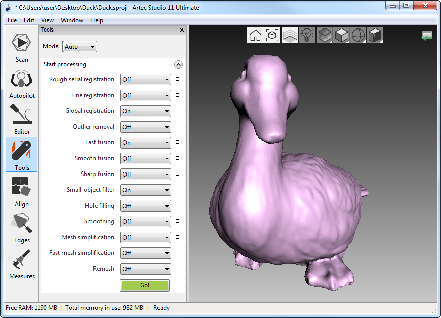
Figure 119. The extended Auto postprocessing menu.
To switch from manual to automatic mode, open the Tools panel and choose the Auto option from the dropdown list in the left corner. Click the button near Go! to view all options available in automatic mode. Note that only Global registration, Fast fusion and Small-object filter are enabled by default. To perform other actions automatically, choose the On option in the dropdown list next to the required function, or choose Off to exclude a function from automatic processing. Click Go! or hit Ctrl + G to begin automatic processing.
Each algorithm setting and parameter is based on the values for manual mode. To change these values, switch to Manual mode, make the necessary alterations and then run automatic processing—Artec Studio will apply all changes.
Keep in mind that the algorithms run in the order in which they are listed, starting with Rough serial registration and ending with Remesh. Thus, if you want to run the Small-object filter before Fast fusion or Global registration, for instance, you must do so manually.
Unlike manual processing, automatic processing runs without the need for constant user attention, so it is more convenient when processing large objects: you can configure the settings, start the process and leave it unattended. It can also process objects of any size, reducing the number of mouse clicks to get the result.
Texturing
Artec scanners are equipped with a color camera, allowing you to capture 3D surfaces with texture and expanding the range of objects available for scanning. Texturing is a process that projects textures from the individual frames onto the fused mesh.
Preliminary Steps
To take advantage of texture, do the following:
- Make sure the Don’t record texture checkbox is cleared.
- Adjust the capture frequency for texture frames (see Texture-Recording Mode) if necessary.
- Avoid turning off the flash bulb.
- Adjust the texture brightness in Preview mode by using the eponymous slider in the Scan panel.
- Scan the object using a tracking algorithm of your choice. Captured frames are marked with the letter “T” in the Workspace panel (surface-view mode) (see Figure 73., right).
- Process the data and create a model, consulting the list in the beginning of Data Processing or Autopilot.
- Run a mesh-simplification algorithm for the resulting model (see Mesh Simplification) to accelerate the texturing process.
- Use the Texture panel to apply the texture to the model.
Applying Texture
The 3D model obtained after fusion contains no texture information. To apply textures onto a model, open the Texture panel and choose a model from the first list (see Figure 121.); Artec Studio will apply the textures to this model. Next, select from the second list the scans from which you created the model (these scans have the required textures).
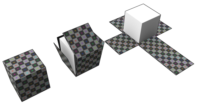
Figure 120. Simplified illustration of texture applying: texture as a single file.
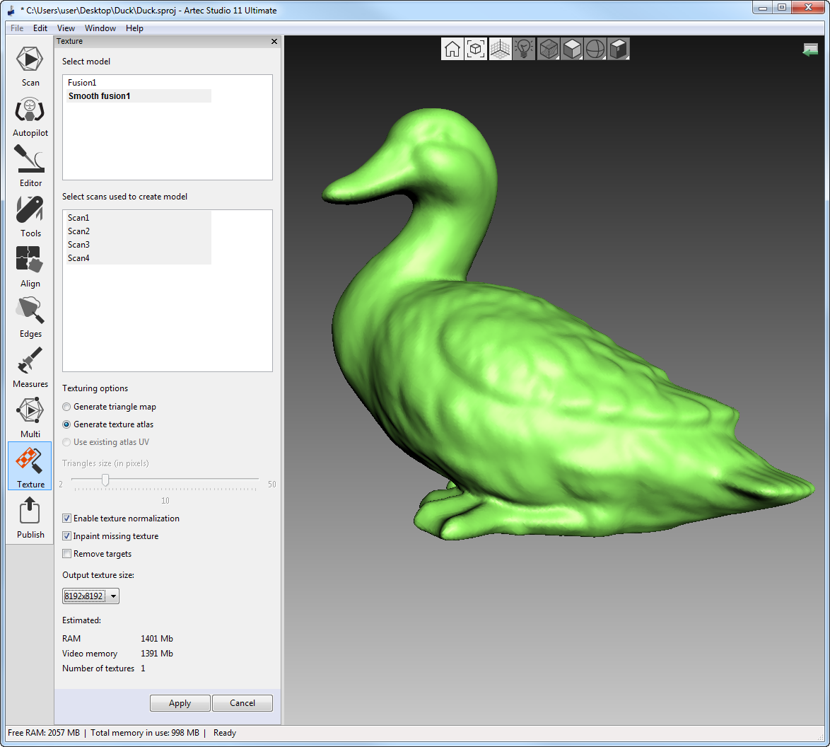
Figure 121. Choosing a texture-application method and adjusting its parameters.
Warning
We recommend that you avoid applying texture to models that have undergone major changes in geometry or orientation. The algorithm will apply the texture incorrectly if you have done any of the following:
- Transform or position the model relative to its source scans
- Nonrigid alignment (see Nonrigid Alignment)
- Erase major parts of the model
Perform these operations only after texturing.
Next, you will need to choose a method for applying textures to the model. Artec Studio offers two methods:
- Generate triangle map
- Generate texture atlas
Generating Triangle Map
The Generate triangle map method transfers all textured triangles to a square texture image (or a series of images). You can adjust the size of the triangles [2] (in pixels) using the Triangle size slider (see Figure 122., right). To select the resulting texture size, use the dropdown list (maximum texture size depends on the capabilities of your graphics card). After changing the triangle/texture size, the estimated number of textures will appear in the Estimated area at the bottom of the panel; the actual number may differ slightly, however.
Generating Texture Atlas
The Generate texture atlas method cuts the surface into pieces, then unfolds and nests these pieces flat and fits them into the specified image size (see Figure 122. (middle) and Figure 62. in Displaying Boundaries of Texture Atlas). This method takes longer to run than Generate triangle map, but the resulting texture is much more convenient for manual editing.
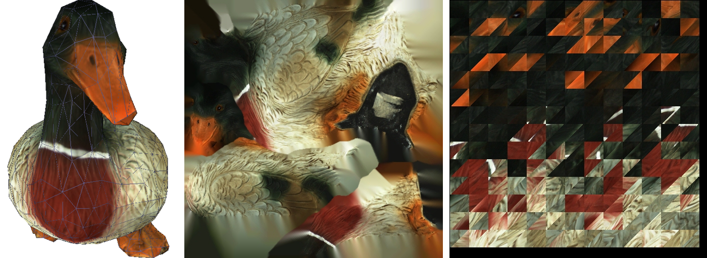
Figure 122. Texture mapping methods: mesh with texture applied (left), texture-atlas sample (middle) and triangle-map sample (right). The latter covers only a portion of the mesh surface (the rest two images not shown).
To modify a texture using an inpainting technique, use one of these two options:
- Inpaint missing texture
- —allows you to apply a texture to regions with no texture information by spreading it from the neighboring regions.
- Remove targets
- —does the same thing, painting out targets by applying surrounding texture information (targets are used to facilitate scanning—see Target-Assisted Scanning). This option makes sense if you enabled remove_targets before producing this fusion model (see Fusion).
- Enable texture normalization
- —this option is selected by default. It aims to compensate for uneven lighting caused by movement of a scanner’s flash unit during capture. We recommend leaving this option enabled.
General Information
Finally, select the required Output texture size and click Apply to start the texture-mapping process.
Important
Texturing with the 16K resolution is only available if your graphics card features at least 3 GB of GPU memory.
To reduce or increase the resolution (Output texture size) of the already applied texture, you can re-apply it several times faster by enabling the Use existing atlas UV option.
| Mode | Texture Distortion | Speed | Number of Textures | Texture-Resolution Management |
|---|---|---|---|---|
| Triangle map | Does not preserve aspect ratio of triangles | Fast | One or more | Adjust triangle size and texture-image resolution |
| Texture atlas | Preserves aspect ratio of triangles | Slow | Only one | Adjust texture-image resolution |
Note that to optimize resource utilization Artec Studio unloads all surfaces from memory, except those needed for texturing, before running the applying procedure. For a more detailed description of selective project-data loading, see Selectively Loading Project Data.
Footnotes
| [2] | Triangle size is determined by the number of pixels per side. |
Texture Adjustment
After the texturing is complete, you can adjust the texture on the model (see Figure 124.).
Note
You can always return to texture adjustment using the Adjust texture command in the Workspace panel’s context menu.
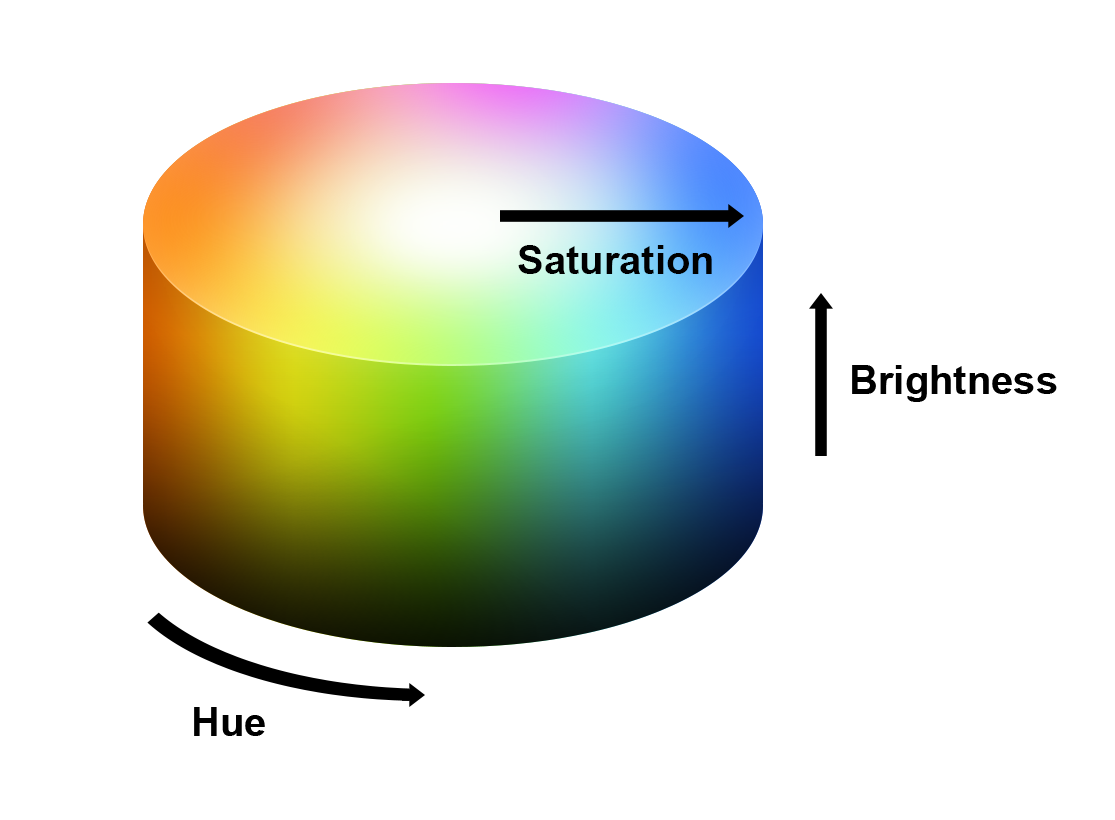
Figure 123. Hue, saturation and brightness representation.
You can adjust the following texture parameters by way of the corresponding sliders (see Figure 123. for details):
- Brightness
- Saturation
- Hue
- Contrast
- Gamma correction
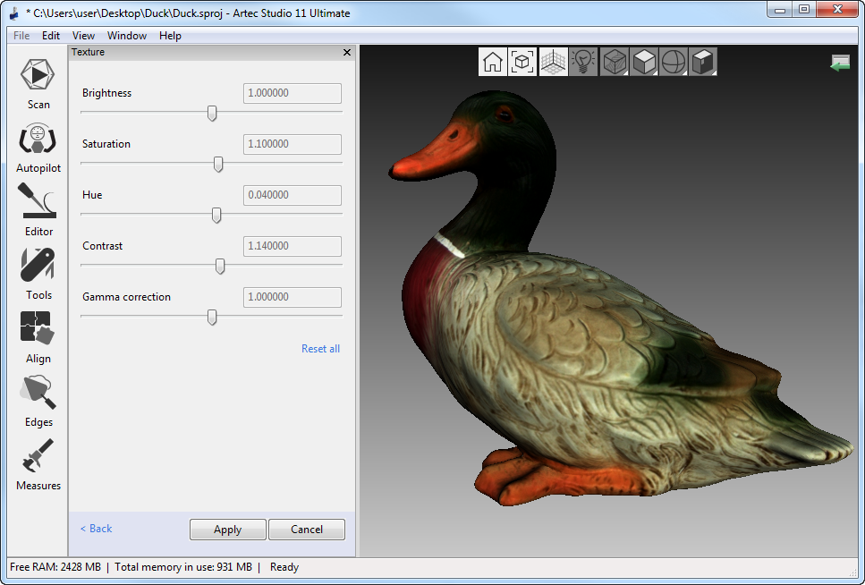
Figure 124. Texture adjustments.
The initial position of the Hue slider corresponds to the current texture color. Dragging it left or right corresponds to rotation counterclockwise or clockwise, respectively, on the color wheel.
After making the necessary changes, click Apply to transfer the resulting textured model to the Workspace panel.
Texture-Healing Brush: Manual Inpainting
You can manually inpaint missing textures by using the Texture-healing brush. This tool is based on the same algorithm as the Inpaint missing texture option covered in Applying Texture. The inpainting algorithm uses texture information from neighboring regions to fill in areas with missing or incorrect texture. Left image in Figure 125. shows a small texture imperfection: a felt-tip pen mark on the figurine. Results of inpainting this region appear in Figure 125. (right).
Important
This version of Artec Studio does not support texture restoration on the models textured using Triangle map method and in regions of any models that have been corrected using the Defeature brush.
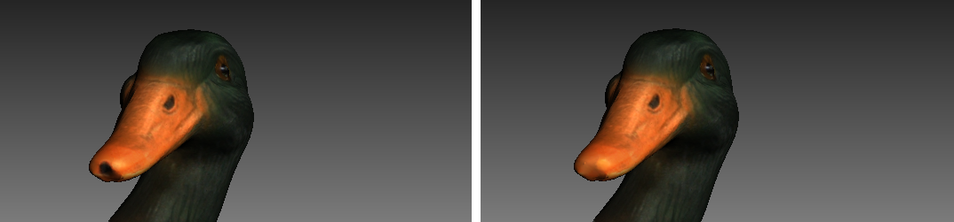
Figure 125. Texture-healing brush: before application (left) and after (right).
To launch the tool and inpaint a texture, do the following:
Make sure the model that you intend to edit is marked with the
icon.Open the Editor panel by clicking its icon in the side toolbar.
Select the Texture-healing brush by clicking the
icon.Note
Make sure the Select through toggle appears as
in the 3D View window.Select a mode: 2D selection or 3D selection.
Hold down
Ctrlwhile usingScroll wheelor[and]keys to adjust the tool size. It should not exceed the size of the region that needs texture correction.Paint over the region of interest using
LMBwhile holding downCtrlso that the tool (a circle or a spot) only rolls over the problem area. Try to avoid touching neighboring areas.Click Apply to accept the changes or Cancel to reject them.
Note
If you paint an area in which the number of polygons exceeds the value specified in the settings dialog (see Warnings), a message will appear prompting you to either ignore the value, which means that processing may take longer, or cancel the operation.